This unit focuses on the last stages of compilation, namely turning an AST into executable machine code. As we will see, modern compilers almost never go directly from a program’s AST to a specific machine code like ARM or x86; rather, they translate to a compiler-specific intermediate language, which is somewhat like assembly code, but with important differences. That intermediate language can then be subsequently optimized and translated to the target CPU’s machine instructions.

This unit mostly focuses on what that intermediate language looks like, how it differs from machine code, and why it is useful for making later performance optimizations.

We could spend an entire course on this, and indeed there are undergraduate courses that really focus on this “back-end” of the compiler and the many interesting and brilliant ideas that have gone into developing compiler optimizations and internal representations. The scope of our discussion will mostly be on the translation into intermediate representation, with just a “hint” of some optimizations that may happen afterwards.

1 Intermediate Representations

Modern compilers generally work in many phases of analysis, simplification, and optimization. After each stage, the code is in some intermediate representation (IR) internal to the compiler.

The initial stage of IR may be an abstract syntax tree (AST). Indeed, in interpreted languages without much optimization, the AST may be the only IR used.

The bytecode language of various virtual machines, as we just discussed, is another kind of IR. This bytecode is usually a stack-based language, where one of the main goals is to make the bytecode as small as possible while still allowing fast low-level execution. These bytecode languages are often closely tied to the features of the original source code language (e.g., Java bytecode is closely tied to the Java language).

Optimizing compilers nowadays also go through at least one more stage of IR, after the AST, looking closer to the ultimate goal of machine code while still being independent of the target architecture. The kind of IR that compilers use has different goals than ASTs or bytecode: it is designed to be easy to optimize in later steps of the compilation, rather than being targeted towards simplicity or compactness.

We will focus on some properties of an IR which is both language and machine-independent:

• Three-address code (3AC)
• Basic blocks
• Control flow graph (CFG)
• Single static assignment (SSA)

These are the properties shared by some IRs for popular modern compilers, which have the attractive property of being language-independent and machine-independent. That means that you can produce this IR from any initial programming language source code, and from this IR you can produce actual machine code for many different target architectures.

2 LLVM and clang specifics

In our upcoming double lab, we will look at compiling SPL source code to the IR for LLVM, the modern compiler suite behind clang and clang++. The IR properties we cover here are very similar to those found in the LLVM IR, so will be relevant to your work in that lab.

If you want to see the LLVM IR in action, there are a few useful clang commands you can use:

• Install needed tools: This should already be installed on the lab machines, but on your own laptop (Ubuntu VM or WSL) you can run:

  roche@ubuntu$ sudo apt update
  roche@ubuntu$ sudo apt install clang llvm

• View Clang’s AST of C code: Remember that this part of compilation is really turning an AST into some IR language representation. If you are curious, you can see the abstract syntax of a C program in clang by running

  roche@ubuntu$ clang -Xclang -ast-dump yourprogram.c

• Translate C into LLVM IR: This is probably the most useful way to really learn what LLVM IR code looks like and how it works. The output will be saved in a .ll file like yourprogram.ll:

  roche@ubuntu$ clang -S -emit-llvm yourprogram.c # creates yourprogram.ll

• Run LLVM IR directly: There is a handy utility lli which can directly interpret LLVM IR, like

  roche@ubuntu$ lli yourprogram.ll # creates yourprogram.s

• Translate LLVM IR to assembly: To see what the actual machine assembly code would be for some LLVM IR, you can use the llc tool, which creates an assembly file with a .s extension like yourprogram.s.

  roche@ubuntu$ llc yourprogram.ll # creates yourprogram.s

• Turn LLVM IR (or assembly) into an executable: You can just use the clang command to turn any .c C source code, or .ll LLVM IR program, or .s assembly, into an executable program like a.out:

  roche@ubuntu$ clang yourprogram.ll # creates a.out

3 Three-address code

A three-address code, abbreviated 3AC or TAC, is a style of IR in which every instruction follows a similar format:

destination_addr = source_addr1 operation source_addr2

Some operations in 3AC have fewer than 3 addresses, but usually not more. This is quite similar to many basic machine instructions like ADD or MUL, but it’s important to emphasize that a 3AC IR is still machine-independent and will usually be simpler than a full assembly language like x86 or ARM.

Sometimes (confusingly) the instructions of a 3AC are called “quadruples”, because they really consist of four parts: the operation, the destination address, and the two (or sometimes one) source addresses.

The number of operations is usually relatively small compared to a full programming language. For example, you wouldn’t probably have a += operator to add and update a variable; instead you would have to use addition where the destination address matches the first source address.

Like assembly code, 3AC languages don’t usually have any looping or if/else blocks. Instead, you have goto operations and labels. In the LLVM IR we will use, an unconditional branch looks like

br <label>

and in a conditional branch we see the more typical 3AC structure:

br <condition_addr> <label1> <label2>

In the conditional branch, condition_addr is the address of a boolean value. If that value is 1 (i.e., true), then the code jumps to label1, and otherwise it jumps to label2.

An example is in order! Consider this simple Python code fragment to compute the smallest prime factor p of an integer n.

p = 2
while p*p <= n:
    if n % p == 0:
        break
    p += 1
if p*p > n:
    p = n
print(p)

Now let’s see how that might translate into 3AC:

    p = 2
condition:
    temp = p * p
    check = temp <= n
    br check loop afterloop
loop:
    temp = n % p
    check = temp == 0
    br check afterloop update
update:
    p = p + 1
    br condition
afterloop:
    temp = p * p
    check = n < temp
    br check if2 afterif
if2:
    p = n
    br afterif
afterif:
    # Note: this is one plausible way a library call could work,
    # assuming some special variable names arg1, arg2, etc.
    arg1 = "%d\n"
    arg2 = p
    call printf

Notice that it got quite a bit longer - that’s typical, because we have to take something that used to be on one line like if p*p > n, and break it into multiple statements. This also involves adding some new variables which didn’t exist in the original program. In this case, we added new variables temp and check as temporaries to store some intermediate computations.

Basic blocks and (the other) CFGs

A useful property of most IRs is that they make it easier for the compiler to analyze the control flow of the program. The way this is typically represented is by first breaking the program into a number of basic blocks - sequential chunks of statements with no branches. In the strictest setting (which the case for LLVM IR that we will see in lab), each basic block must start with a label and end with some control flow statement like a branch or a function call.

The example above is almost in basic block form already, except that we need to give a label to the first block and add an unconditional branch at the end of it:

initial:
    p = 2
    br condition
condition:
    temp = p * p
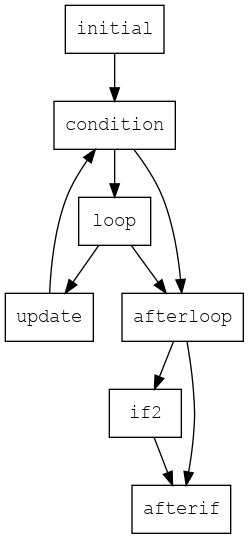
    # ... the rest is the same

Once the program is broken into basic blocks, we can generate the control flow graph (CFG) showing possible execution paths in the program between the basic blocks. Specifically, each node in the CFG is a basic block, indicated by its label, and each directed edge represents a possible execution path from the end of that basic block to another one.

(Note: CFG is now an overloaded term in this class, because it also stands for Context-Free Grammar in the context of parsing. Hopefully the context (haha) will make the distinction clear.)

Here is the CFG for the prime factor program above:

4 SSA

The final aspect of the modern IRs (including the LLVM IR) that we will look at is called static single assignment, or SSA. This is a restriction in how variable or register names are assigned in the IR which makes many later compiler optimizations much easier to perform. Interestingly, SSA is very closely related to the concept of referential transparency that we learned from functional programming.

Here’s the formal definition:

A program is in SSA form if every variable in the program is assigned only once.

That is, any name can appear on the left-hand side of an assignment only once in the program. It can appear many times on the right-hand side (after the assignment!), but only once on the left-hand side. This model is also called write once, read many.

Let’s recall our running example of the prime factor finding program, in 3AC form:

initial:
    p = 2
    br condition
condition:
    temp = p * p
    check = temp <= n
    br check loop afterloop
loop:
    temp = n % p
    check = temp == 0
    br check afterloop update
update:
    p = p + 1
    br condition
afterloop:
    temp = p * p
    check = n < temp
    br check if2 afterif
if2:
    p = n
    br afterif
afterif:
    # Note: this is one plausible way a library call could work,
    # assuming some special variable names arg1, arg2, etc.
    arg1 = "%d\n"
    arg2 = p
    call printf

This is currently not in SSA form, because the variables p, temp, and check are reassigned in a few places.

The usual fix is to replace each reassignment with a new variable name, so that they never get reused and we have good ol SSA form back again. We’ll replace each assignment of p with p1, p2, etc., and change each subsequent usage of temp and check to t1, t2, etc.:

initial:
    p1 = 2
    br condition
condition:
    t1 = p * p  ## PROBLEM
    t2 = t1 <= n
    br t2 loop afterloop
loop:
    t3 = n % p  ## PROBLEM
    t4 = temp == 0
    br t4 afterloop update
update:
    p2 = p + 1  ## PROBLEM
    br condition
afterloop:
    t5 = p * p  ## PROBLEM
    t6 = n < t5
    br t6 if2 afterif
if2:
    p3 = n
    br afterif
afterif:
    arg1 = "%d\n"
    arg2 = p    ## PROBLEM
    call printf

Great! This now follows the SSA form wherein each variable name is assigned only once, except there are some problems very subtly identified in the code above. Take a second to see if you can figure out what the trouble is here.

The problem is, now that we’ve changed all the reassignments of the original variable p to p1, p2, and p3, how do we know what each usage of p refers to on the right-hand side? Take for example the first problem:

t1 = p * p

You might be tempted to say that p here should be p1, from the initial block. And sure, that’s what p will be the first time around. But the next time the condition block is executed, it’s not coming from the initial block but rather from the update block, so at that point p should be p2.

In other words, the value p in this line could be coming either from p1 or p2, depending on where the program actually is in its execution. This was not a problem with the temp and check variables that we replaced with t1, t2, and so on, because their uses were within the same basic block where the variable was set, so there wasn’t any question.

But p is essentially acting as a conduit for communication between the basic blocks, being set in one block and accessed in another.

Now, there are two basic ways to solve this. The “easy way” is to use memory: for any variable like p which has some ambiguous uses, we simply store p into memory (on the stack), and load its value from memory each time it is used. Then we only need to save the address of p within the variables of the program, and even though p may be changing repeatedly, that address never changes, so the rules of SSA are not violated. In fact, this is the approach we will take in our LLVM IR lab.

But using memory this way is very costly in terms of computing time. Each load or store from RAM (or even cache) is hundreds or thousands of times slower than reading from a CPU register. So we would really like to keep these values as variables in our 3AC code, if possible, to allow the later stages of compilation to potentially store them in CPU registers and make the program as fast as possible.

The solution to this, the “hard way”, is to use what is called a phi function, written usually with the actual Greek letter \(\phi\). A phi function is used exactly in cases where the value of a variable in some basic block of the program could come from two or more different assignments, depending on the control flow at run-time. It just means adding one more assignment to the result of the \(\phi\) function, and the arguments to the phi function are the different possible variables whose value we want to take, depending on which variable’s basic block was most recently executed.

I know - that description of the phi function seems convoluted. That’s what makes this the “hard way”! But it’s how actual compilers work, and it’s not too hard to understand once we see some examples. For the case of the assignment t1 = p * p in our running example, we would replace this with

p4 = phi(p1, p2)  # gets p1 or p2 depending on control flow
t1 = p4 * p4    # Now we can use p4 multiple times in SSA form

Applying this idea throughout the program yields this complete description of our prime factor finding code, in proper SSA form:

initial:
    p1 = 2
    br condition
condition:
    p4 = phi(p1, p2)
    t1 = p4 * p4
    t2 = t1 <= n
    br t2 loop afterloop
loop:
    t3 = n % p4
    t4 = t3 == 0
    br t4 afterloop update
update:
    p2 = p4 + 1
    br condition
afterloop:
    t5 = p4 * p4
    t6 = n < t5
    br t6 if2 afterif
if2:
    p3 = n
    br afterif
afterif:
    p5 = phi(p3, p4)
    arg1 = "%d\n"
    arg2 = p5
    call printf

Ultimately, we needed only two phi functions to get this program working. How did we figure this out - when to use a phi function and when not to, or which version of p to use in each right-hand side?

Generally, this is what you have to do to figure out what any given variable reference should be replaced with in SSA form:

1. If the variable was set earlier in the same basic block, use that name. For example:

   y = 7 * 3
   y = y + 1
   temp = y < 10

   becomes simply

   y1 = 7 * 3
   y2 = y1 + 1    # y1 is the most recent defn in the same basic block
   temp = y2 < 10 # y2 is the most recent defn in the same basic block

2. If the variable was not set earlier in the same basic block, then trace backwards all possible paths in the control flow graph, moving backwards until we find the most recent setting of the variable in each path that could have reached this basic block.

   If all paths reach the same basic block where the variable was most recently set, use that variable name. For example:

   one:
       x = 5
       x = x - 3
       br x two three
   two:
       y = x * 10
       br three
   three:
       y = x + 20

   becomes

   one:
       x1 = 5
       x2 = x1 - 3     # same basic block reference
       br x2 two three # same basic block reference
   two:
       y1 = x2 * 10    # x most recently set in block one
       br three
   three:
       y2 = x2 + 20    # x most recently set in block one

3. Finally, if cases (1) and (2) both fail, then we need to have a phi funciton. Tracing backwards through the CFG, we find all basic blocks along execution paths where the variable could have been most recently set. Then we make a new variable and set it to phi of all of those possible variable values. For example, slightly changing the previous situation:

   one:
       x = 5
       x = x - 3
       br x two three
   two:
       x = x * 10
       br three
   three:
       x = x + 20

   becomes

   one:
       x1 = 5
       x2 = x1 - 3     # same basic block reference
       br x2 two three # same basic block reference
   two:
       x3 = x2 * 10    # x most recently set in block one
       br three
   three:
       x4 = phi(x2, x3)  # x could come from block one or two
       y2 = x4 + 20    # now we use x4

5 Optimizations

At this point, you should be asking “WHY!!!” Why did we do all this work to convert to the 3AC SSA Intermediate Representation and draw the CFG?

The main answer is that this representation makes it much easier for the compiler to perform code optimizations in later steps. Some examples of these optimizations are:

• Constant propagation
• Common subexpression elimination
• Dead code elimination
• Code motion
• Function inlining
• Loop unrolling
• Strength reduction
• Register allocation

Depending on timing, we may have a chance to look at a few of these in more detail.