This is the archived website of SI 335 from the Spring 2013 semester. Feel free to browse around; you may also find more recent offerings at my teaching page.
Readings
- CLRS, Sections 22.1-22.4, 24.2-24.3, 25.1-25.2, and 35.2.
- DPV, Sections 3.1-3.3, 4.4-4.5, 5.1, 6.1, 6.6, and 9.1-9.3
Algorithms: in python
- Slides: note-taking version
- These notes: printable version
Beginning of Class 31
1 Graphs
NOTE: All this section should be review from Data Structures!
Graphs (sometimes called "networks") are an extremely useful and versatile way of representing information. At its core, a graph is a collection of items (the nodes) and relationships between them (edges). Here is a very small sampling of different kinds of information that can be represented with a graph:
- Cities in a country or continent and the highways that connect them. Can be used by services like Google Maps to tell you the fastest way to get somewhere.
- People in an organization and the relationships between them
- ("boss", "acquaintance", "friend", etc.).
- Computers and servers in a network and the connections between them. Problems we might ask are how to get a message from one machine to another and how to best configure the network for redundancy if one machine goes down.
- Web pages and the hyperlinks between them
- Dependencies in a Makefile
- Scheduling tasks given some constraints (like "A has to happen after B" or "A and B can't happen simultaneously".)
Because of this, graphs rightfully belong to the class of basic computational structures alongside other things like numbers, lists, and collections. We'll examine a few of the most important algorithms and problems with graphs but there are many, many more that arise in all kinds of varied circumstances.
1.1 Definitions and Terminology
A graph \(G=(V,E)\) is a tuple of "nodes" or "vertices" in the set V, and "edges" in the set E that connect the vertices. Each edge goes between two vertices, so we will write it as an ordered pair \((u,v)\) for \(u,v\in V\). If G is a weighted graph, then there is also a "weight function" \(\omega\) such that \(\omega(u,v)\) is some non-negative number (possibly infinity) for every edge \((u,v)\in E\).
For convenience we will always write \(n=|V|\) for the number of nodes and \(m=|E|\) for the number of edges in a graph. You can see that \(m\leq n^2\), and if the graph doesn't trivially separate into disconnected pieces, then \(m\geq n-1\) as well. We say that a graph is "sparse" if m is close to n, and a graph is "dense" if m is closer to \(n^2\). (Yes, this is a bit fuzzy!)
The most general kind of graph we will examine is a directed, weighted, simple graph. The "directed" part means that the edges have arrows on them, indicating the direction of the edge. And a "simple" graph is one that doesn't allow repeated edges (in the same direction, with the same endpoints) or loops (edges from a node back onto itself).
Time for an example: Human migration (immigration) between countries. Each vertex in the graph is a location (country, region, state) and an edge represents people moving from one location to another. The weight on each edge is the number of people that made that move in some given time frame. Rather than me try and make a pretty picture here, why don't you look here, here, or here — look at page 11.
From this general picture we can have simplifications. An unweighted graph is one without weights on the edges, which we can represent as a weighted graph where every edge has weight 1. Unweighted graphs are common when the relationships represented by edges constitute "yes/no" questions. For example, in a web graph the nodes might be web sites and the edges mean "this page links to that page".
There are also undirected graphs, which we can represent as a directed graph in which every edge goes in both directions. That is, \((u,v)\in E \Leftrightarrow (v,u)\in E\). Undirected graphs might indicate that there is no hierarchical difference between the endpoints of an edge. For example, a computer network graph with edges representing a point-to-point connection with a certain bandwidth might be undirected.
Of course some graphs are also undirected and unweighted. For example, we could have a graph where each vertex is a Midshipman and an edge between two Mids means they are in a class together.
This might also be a good time to mention an important detail: weighted graphs are often complete. A complete graph is one in which every possible edge exists. For example, in the migration flow graph, we can always draw an edge from one country to another, even if the weight on the edge might be 0 (meaning no migration in that direction).
1.2 Representations
How can we store a graph in a computer? We need to represent the vertices V and the edges E. Representing the vertices is easy: we just assign them numbers from 0 up to \(n-1\) and use those numbers to refer to the vertices. Perhaps the labels (example: country name) are stored in an array by vertex index.
The tricky part is how to store the edges. We will at various points consider three fundamental ways of representing edges:
Adjacency Matrix. an \(n \times n\) array stores at location
A[i][j]the weight of the edge from vertex i to vertex j. Since we have to specify a weight for every single edge, we usually choose some default value like 0 or infinity for the weight of an edge that isn't actually in the graph. The size of this representation is always \(\Theta(n^2)\). Generally works well for dense graphs.Adjacency List. For each vertex u, we store a list of all the outgoing edges from u in the graph (that is, all edges that start at u). These edges are represented by a pair \((v,x)\), where \((u,v)\) is an edge in the graph with weight x. So the overall representation is an array of lists of pairs. One list for each vertex, one pair for each edge. In an unweighted graph, we can just store the index of the successor vertices v rather than actual pairs. The size of this representation is always \(\Theta(n+m)\). Generally works a bit better for sparse graphs because this representation uses less space when m is much smaller than \(n^2\).
Implicit. This is similar to the previous representation, except that rather than storing the array of lists explicitly, it is implicitly given by a function that takes a node index and returns the list of outgoing edges from that node. This is really important for huge graphs that couldn't possibly stored in a computer, like the web graph. We can even have infinite graphs (!) in this representation.
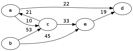
Example 1
For the example above, we would first number the nodes a-e as 0, 1, 2, 3, 4. Then the adjacency matrix representation would be:
\[ \begin{array}{c*{5}{|c}} & 0 & 1 & 2 & 3 & 4 \\ \hline 0 & 0 & \infty& 10 & 22 & \infty\\ \hline 1 & \infty&0 & 53 & \infty& 45 \\ \hline 2 & 21 & \infty& 0 & \infty& 33 \\ \hline 3 & \infty& \infty& \infty& 0 & \infty\\ \hline 4 & \infty& \infty& \infty& 19 & 0 \end{array} \]
Notice that the entries on the main diagonal (like the weight of a node from an edge to itself) were all set to 0, and the entries corresponding to edges not in the graph were set to \(\infty\). This is just a choice which would depend on the application. For example these choices would make sense if the edges represent distances between nodes.
The adjacency list representation, on the other hand, would be something like
[( (2,10), (3,22) ),
 ( (2,53), (4,45) ),
 ( (0,21), (4,33) ),
 ( ),
 ( (3,19) )
]
1.3 General Search
Often we want to explore all the nodes and edges in a graph, in the search for a certain node or path in the graph. There are a variety of ways to accomplish this that follow the following basic template:
def genericSearch(G, start, end):
    colors = {}
    for u in G.V:
        colors[u] = "white"
    # initialize fringe with node-weight pairs
    while len(fringe) > 0:
        (u, w1) = fringe.top()
        if colors[u] == "white":
            colors[u] = "gray"
            for (v, w2) in G.edgesFrom(u):
                if colors[v] == "white":
                    fringe.insert((v, w1+w2))
        elif colors[u] == "gray":
            colors[u] = "black"
        else:
            fringe.remove((u, w1))
There are a few big blanks in this template:
- How to initialize the
fringe. It will usually be initialized with at least one node, with weight zero. - What should the algorithm return or produce? Often something special will happen either right after a node is colored gray ("pre-visit") or right after it is colored black ("post-visit"). In fact, the post-visits is the only reason why we have gray nodes at all!
- How to insert into the
fringe - What data structure to use for
fringe. This actually makes a huge difference on what the algorithm does.
The most common thing we want to use this algorithm for is to search in a graph for a path between two given vertices. Recall that a path in a graph of length k is just a list of \(k+1\) vertices \((u_0, u_1, \ldots, u_k)\) such that every \((u_{i-1},u_i)\) is an edge in the graph. (The weight of the path is just the sum of those edge weights.)
To searching for a path between two vertices, the fringe is initialized with the initial path vertex, and weight zero. That's (a) from the template. For (b), we add a simple pre-visit check if u (the vertex just popped from fringe) is equal to the final path vertex. If so, the search is complete, and the weight w1 is the weight of the path found from the initial to the final vertex. Also, for a basic search where we're not trying to find minimal paths or anything, the fringe.update(...) just means inserting the new node-key pair into the collection wherever it's supposed to go.
What about (d) in the template, the data structure to use for the fringe? If we use a last-in/first-out stack, then we get a "depth-first search" (DFS) that completely explores all the descendants of each node before moving on to the next one. If a first-in/first-out queue is used instead, we get a "breadth-first search" (BFS) that explores all the nodes a certain number of hops away from the initial vertex before moving on.
The pseudocode linked from this page has a specification of the DFS and BFS algorithms in detail.
For example, in the directed graph above, there are two paths from a to d: \((a,d)\) with weight 22, and \((a,c,e,d)\) with weight \(10+33+19=62\). Assuming that edges are explored in numerical order in the for loop in the search algorithm, a DFS will return the length-3 path while a BFS will always return the length-1 path.
Beginning of Class 32
2 Applications of Search
Let's look at a few more examples of this basic search recipe in action. See the textbooks for many more.
2.1 Linearizing a DAG
A "cycle" in a graph is a path that starts and ends at the same vertex, so it goes around in a loop. An important subclass of graphs is those that don't have any cycles. In other words, they're acyclic. We already have a word for a (connected) undirected graph with no cycles: a tree. (If it's not connected, it's called a forest.)
The extension to directed graphs is much more varied than trees, but with a much less interesting name: directed acyclic graph, or "DAG". Such graphs come out of numerous applications where a cycle would be impossible or problematic. For example, any biological population forms a dag from parent-child relationships. It can't have any cycles because that would mean someone is their own parent or grandparent or great-grandparent, an impossibility due to the flow of time.
Another example of a DAG is that formed by the dependencies between software packages in a large software repository such as debian (for free and open-source Linux software). The idea is that of software reusability and composability.
Say I'm writing a new program to do RSA encryption and decryption, but I don't want to have to write my own package for multiple-precision arithmetic. No problem — I can just say that my software package depends on an existing multi-precision integer package such as libgmp.
More generally, if Package A depends on Package B, then Package B must be installed before A can be. Besides its own code, each package comes with a list of its own dependencies.
Now this brings up a problem: given a big list of packages, how to order them, and all their dependencies, and their dependencies' dependencies, so that every package is installed only once, and before it is needed by another package? Let's put this problem in graph theory terms:
Problem: DAG Linearization
Input A DAG \(G=(V,E)\).
Output An ordering of the n vertices in V as \((u_1,u_2,\ldots,u_n)\) such that every edge in E is of the form \((u_i,u_j)\) with \(i\lt j\).
(Sometimes — your textbook for instance — this is called "topological sort", but I'm not using that term because this really has nothing to do with sorting an array, and because you have no idea what topology is.)
Some other applications of this problem besides installing software packages are:
- Scheduling tasks with dependencies. For example, to cook an omelette I have to beat some eggs, chop some veggies, heat up the pan, and so on. Now these things can't happen in any order: for example, the veggies have to be chopped and the pan has to be hot before I add the veggies to the pan. Linearization provides an order to execute these tasks that honors the constraints I've given. Same problem with scheduling classes that have prerequisites or scheduling a workout so you don't tire out certain muscle groups too quickly.
- Constructing a dynamic programming algorithm. Remember that dynamic programming works by identifying a whole mess of subproblems, and only computing (and saving) the solution to each subproblem once. The tricky thing was figuring out the ordering so that whenever the solution to some subproblem is needed, it's already been computed. The dependencies between subproblems forms a DAG, and a linearization provides a valid ordering.
So this is a pretty useful problem! How do we do it? The solution is to build up the ordered list of vertices in the post-visit step of a DFS. The reason it works is that, once we get to the post-visit stage for a node in a DFS, it means that all its descendants have been completely explored. If all those descendants have already been added to the ordered list, we just need to make sure this vertex is before all those in the list; so add it to the front. Here's the template, filled out for the linearization problem:
def linearize(G):
    order = []
    colors = {}
    fringe = []
    for u in G.V:
        colors[u] = "white"
        fringe.append(u)
    while len(fringe) > 0:
        u = fringe[-1] # back of the list; DFS
        if colors[u] == "white":
            colors[u] = "gray"
            for (v,w2) in G.edgesFrom(u):
                if colors[v] == "white":
                    fringe.append(v)
        elif colors[u] == "gray":
            colors[u] = "black"
            order.insert(0, u)
        else:
            fringe.pop()
    return order
Do you see where the template has been filled-in? The only lines that have changed are 1, 3, 4, and 14.
Let's see how this works on an example. Given the following DAG:
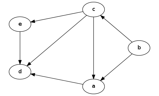
A DAG
The linearize algorithm will order this DAG as follows, from left-to-right:
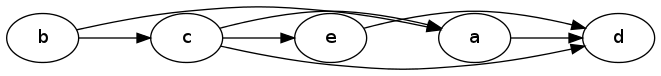
Linearized Dag
Notice that the relative ordering of nodes a and e doesn't really matter; it just depends on which one gets explored first in the DFS.
To see why this is really true, we need to prove some lemmas. Actually these lemmas apply to any kind of DFS, not just the algorithm above to do linearization. The first one has to do with parent-child relationships within the nodes of the stack:
Lemma: For any vertex u in the
fringestack, the first gray vertex v below u in the stack has an outgoing edge to u, \((v,u)\).Proof: This is true at the beginning of the algorithm, since there is only one vertex in the stack.
Now notice that the only place new vertices are added to the stack is on line 10. At this point in the algorithm, there is a vertex u which has just been colored gray, and we are only adding white vertices v that are children of u. So for every new vertex added, the first gray vertex below it in the stack will be u, and therefore the lemma holds for every newly-added vertex.
All that's left is to observe that the colors of vertices are only changed when they are at the top of the stack. When a vertex goes from white to gray or gray to black, it's at the top of the stack, so changing its color won't make the lemma become false.
Therefore because the lemma is true at the beginning, and it stays true whenever the stack or the colors change, so we conclude that the lemma is always true.
What this means is that the gray vertices in the stack at any given time always form a path. This is important because it let's us relate what's special about a DAG to the DFS algorithm: no path can contain the same vertex twice (that would make a cycle). Here's the lemma we get, which again applies to any DFS on any DAG.
(Recall that the descendants of a node u are those vertices v for which there is a path from u to v in the graph. We also say that v is reachable from u.)
Lemma: If G is a DAG, then every time a vertex is colored black on line 13, all its descendants have already been colored black.
Proof: The first fact we need to use is that, if v is a descendant of u, then either v is a child of u (i.e., there is an edge from u to v), or else v is a descendant of some child of u. I'm not going to write down a full proof of this fact, but you could prove it by using induction if you wanted to.
Because of this fact, all we really need to say is that when a vertex is colored black on line 13, all its children have already been colored black. By induction, and using the previous fact, it follows that all the node's descendants are already colored black.
The second fact we need is that, because G is a DAG, I claim that every child node v examined during the for loop on line 9 is either colored white or black. The reason is that, if v were gray, then it must be in the stack somewhere, since nodes are only colored gray when they're already in the stack, and they're only removed from the stack after they've been colored black. But if v is a gray node in the stack, then the previous lemma tells us that there is a path from v to u. This is a contradiction, because the edge from u to v then completes a cycle, which must not exist in any DAG. So every v in the for loop is either white or black.
Now what do we know about a node u when it gets colored black on line 13? It must be colored gray, and it must be at the top of the stack. When it was colored gray on line 8, the following for loop added all its white-colored child vertices above it in the stack. All of those vertices must have been removed from the stack (otherwise how could u get back to the top?), and vertices are only removed on line 15, after they have been colored black. So all its children which were colored white at that time must now be colored black. But we know from the previous fact that all its other children must have been colored black already!
Therefore when a node is colored black on line 13, all its children have already been colored black, and by induction so have all of its descendants.
This is really why the linearize algorithm works. Every vertex is added to the "order" list just as it is colored black. So from the previous lemma, we know that every node will come before all its descendants in the ordered list. And this is exactly what we need to be true in order for the ordered list to have only "forward edges" from earlier vertices in the list to later ones.
2.2 Dijkstra Algorithm
Dijkstra's Algorithm is the most famous application of our basic graph search template, and probably one of the most widely-used non-trivial algorithms in practice. You already saw it in Data Structures, but it's worth looking at again to make sure you really get it.
The idea is to use a different kind of data structure for the fringe, namely a priority queue. This way, at each step, we are choosing the shortest path among all the unexplored (white) vertices in the fringe. What we will get is the (lengths of the) shortest paths from the source vertex u to every other vertex in the graph. For this reason, this is called a single-source shortest paths algorithm.
Beginning of Class 33
The full details will come later, when we specify the data structure for the priority queue. The key difference will be how inserting new nodes into the fringe works.
Besides such updates, let's examine how Dijkstra's algorithm differs from the general search template:
- The
fringeis a priority queue (this is the most important distinction from BFS or DFS!) - There are no gray nodes! Colors go immediately from white to black. This is because there is no "post-processing" phase like with DFS.
- Every time a white (unexplored) node is removed from
fringe, the shortest path to that node has been found. The current version just prints the lengths of these shortest paths. If we also maintained partial paths as nodes were updated in thefringe, we could modify the algorithm to print the actual shortest paths themselves. - A useful variant in practice is just to find the single shortest path between a given pair of vertices. The only modification required would be to stop after the shortest path to the given destination vertex is found.
What Dijkstra's algorithm really computes is a tree of all the shortest paths from the source vertex u. In class we looked at the shortest-paths graph generated by Dijkstra's algorithm from vertex a in the following graph. The edges that make up the shortest-paths tree are colored red. (This example is undirected for convenience, but Dijkstra's algorithm works equally well on directed graphs.)
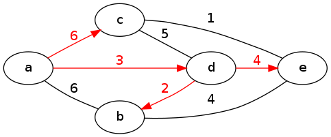
Example for Dijkstra's Algorithm
In order for Dijkstra's algorithm to actually work, it needs to examine all possible paths from the starting vertex in increasing order of path length. This will always happen as long as every time we update a key in the fringe, its key never becomes smaller than anything we've removed from the fringe so far. Look at the algorithm and think about what property would be required to make this true. Since \(w_1\) is the priority of the largest thing we've removed from the fringe so far, and since the updated priority is \(w_1+w_2\), we must have that \(w_1 \le w_1+w_2\), and therefore \(w_2\) must be non-negative. But since this could be the weight of any edge in the graph, we have the following theorem:
Theorem: Dijkstra's algorithm finds the single-source shortest paths in any graph that has only non-negative edge weights.
For the analysis, we have a few things to look at. First let's examine the cost of everything except the operations on fringe. The cost of all this will be dominated by the inner for loop that goes through each node's outgoing edges. In the case of the adjacency matrix graph representation, we have to go through every row of the graph, so the total will be \(\Theta(n^2)\).
If the graph is stored instead as an adjacency list, the TOTAL number of iterations through the inner for loop is exactly m. Since there are n iterations through the outer while loop in either case, the total cost the non-fringe operations in this case is \(\Theta(n+m)\).
As you might recall from Data Structures, the analysis of Dijkstra's algorithm depends on which implementation of the Priority Queue ADT we use for the fringe. The cost will depend on doing n removeMin operations and m update operations. Let's examine two options:
- Heap. Each
updateis just a bubble-up/down, which both cost \(\Theta(\log n)\), and of course everyremoveMincosts the same. So the total cost is \(\Theta((n+m)\log n)\). - Unordered Array. By "unordered" we mean ordered by the index of the node but not by the priority. Here the cost of each
removeMinwill be \(\Theta(n)\), the time to search through the entire array. But (importantly!) the cost of eachupdateis constant, because we don't have to move anything around in the data structure when changing a priority. So the total cost will be \(\Theta(n^2)\).
Here is pseudocode for those two options:
def dijkstraHeap(G, start):
    shortest = {}
    colors = {}
    for u in G.V:
        colors[u] = "white"
    fringe = [(0, start)] # weight goes first for ordering.
    while len(fringe) > 0:
        (w1, u) = heappop(fringe)
        if colors[u] == "white":
            colors[u] = "black"
            shortest[u] = w1
            for (v, w2) in G.edgesFrom(u):
                heappush(fringe, (w1+w2, v))
    return shortest
def dijkstraArray(G, start):
    shortest = {}
    fringe = {}
    for u in G.V:
        fringe[u] = infinity
    fringe[start] = 0
    while len(fringe) > 0:
        w1 = min(fringe.values())
        for u in fringe:
            if fringe[u] == w1:
                break
        del fringe[u]
        shortest[u] = w1
        for (v, w2) in G.edgesFrom(u):
            if v in fringe:
                fringe[v] = min(fringe[v], w1+w2)
    return shortest
Now let's examine the four resulting options for implementing Dijkstra:
\[ \begin{array}{c|c|c|} & {\rm Heap} & {\rm Unsorted\ Array} \\ \hline {\rm Adj.\ Matrix} & \Theta(n^2+m\log n) & \Theta(n^2) \\ \hline {\rm Adj.\ List} & \Theta((n+m)\log n) & \Theta(n^2) \\ \hline \end{array} \]
What does this mean? Well, if we are using the adjacency matrix representation for the graph, we definitely want to use unsorted arrays for Dijkstra's algoritihm. Otherwise, if using adjacency lists, the best choice depends on the sparsity of the graph. But usually we use adjacency lists for sparse graphs, where n is close to m. So usually Heaps are the best choice for Dijkstra's when using adjacency lists.
There is actually a third choice, Fibonacci Heaps, a more sophisticated data structure that can improve the worst-case in some circumstances. We might talk about that data structure later in the course...
Beginning of Class 34
3 All-Pairs Shortest Paths
We now turn to a new problem, which is of course related to some other problems:
Problem: All-Pairs Shortest Paths
Input: A graph \(G=(V,E)\), weighted, and possibly directed.
Output: For every pair of vertices \(u,v\) from V, a shortest (i.e., minimum-weight) path from u to v in the graph.
There are many applications of this problem, and many of them have to do with what I call the "precomputation/query model". Usually we look at algorithms from the standpoint of solving a single problem, once: sort this array, multiply these numbers, etc. But what if we know there will be a number of related problems to solve, perhaps all concerning the same data? Then it is worth the time to analyze that data once (precomputation) so that we can solve the problems that come later (queries) quickly. Essentially, precomputation is about computing all or part of the answer before you need it, so that when you do need it, the answer can be given quickly.
For example, if you were a taxi driver, you would probably want to know the best way to drive between important places like the airport, the Naval Academy, the Pentagon, Bethesda Naval Hospital, Fort Meade, etc. It would be worthwhile to spend some time computing all these optimal routes before actually needing them, so that when needed they can just be recalled quickly. This is in fact essentially what the all-pairs shortest paths problem is doing.
Another classic example is computing routing tables in a static network. If we have any kind of network (for example telephone or LAN) that is not going to change (too frequently), it's more efficient to calculate every optimal route for packets ahead of time rather than on-the-fly as they are needed. Again, the problem boils down to all-pairs shortest paths.
3.1 Repeated Dijkstra
Remember that any time we see a new problem, the first thought should be, "How does this connect to algorithms/problems that I already know about?" In the case of all-pairs shortest paths, the connection is I think pretty obvious: how does this relate to the single-source shortest paths problem?
Recall that the single-source shortest paths problem seeks the shortest paths from a single source vertex u to every other vertex in the given graph. This leads to an initial solution to the all-pairs shortest paths problem: run a single-source shortest paths algorithm multiple times, starting from every possible source vertex in the graph.
Since there are n possible source vertices, this solution will require us to run the single-source shortest path algorithm exactly n times. (Actually, we can get away with \(n-1\) times if the graph is undirected — do you see why?) The algorithm of choice for single-source shortest paths is of course Dijkstra's, so the total cost will be n times the cost of Dijkstra's algorithm.
Now recall that there are a few options for implementing Dijkstra's algorithm. Although there are really four possibilities, we can simplify it down to two cases. If the graph is sparse (meaning the number of edges m is close to the number of vertices n), then we should use the adjacency list representation for the graph and use a min-heap in the algorithm, for a total cost of \(\Theta(n(n+m)\log n)\). If the graph is dense (meaning the number of edges is closer to \(n^2\)), then it is better to use the adjacency matrix representation of our graph and an unsorted list as the priority queue data structure in Dijkstra's algorithm. This will result in a total cost of \(\Theta(n^3)\) for the all-pairs shortest paths problem.
For the remainder of our discussion on all-pairs shortest paths, we're going to focus on algorithms for dense graphs. So we can think of the cost of the "repeated Dijkstra's" approach as just being \(O(n^3)\), for simplicity.
3.2 Storing Paths
An important factor in a successful implementation of any algorithm is the space usage of that algorithm. And certainly the algorithms for this problem are no exception.
Normally when we are discussing and presenting algorithms for these shortest-path problems (such as Dijkstra's), we just talk about computing the lengths of the shortest paths. This captures the essence of the algorithm without making the pseudocode too messy, so it's easier (hopefully) to understand what's going on and to do the analysis.
But in reality of course we want to get the actual paths! So let's consider the size of the paths for the all-pairs shortest paths problem: There are \(n(n-1)\) paths to consider (the number of pairs of vertices), which is \(\Theta(n^2)\) of course, and each path can have at most \(n-1\) edges. So the total size of all the paths is \(\Theta(n^3)\) — same as the time cost of the repeated Dijkstra's algorithm.
In general, this is a bad thing. You should remember from architecture that memory accesses in a computer are much, much more expensive than basic arithmetic computations in the CPU. So if the number of primitive operations in our program is roughly equal to the number of memory accesses, the program is going to be a lot slower than might be suggested just by looking at the time complexity. Sometimes this is referred to as hitting the "memory wall" or having a "memory-bound computation".
Fortunately, there is an easy fix here to bring down the size of the storage. Rather than store the entire path for every possible pair of vertices, we will just store the first node in the path for every pair of vertices. This just requires one more matrix the same size as the adjacency matrix itself. So for example, is the shortest path from a to b is \((a,c,f,d,b)\), then all we store at the \((a,b)\)'th entry in the paths matrix is c, the first vertex along this path. The rest of the path can be constructed by looking at the first vertex in the shortest path from c to b (which is f), then in the shortest path from f to b, and so on. This essentially creates \(\Theta(n^2)\) linked lists within a single n by n matrix. The total storage is just \(\Theta(n^2)\).
So for the algorithms that follow, imagine that we are using this kind of representation to store the shortest paths. Since we know any all-pairs shortest paths algorithm must take at least \(\Omega(n^2)\) time on dense graphs (why?), the size of memory shouldn't dominate these computations. Now, for simplicity, we'll just talk about computing the lengths of the shortest paths, but the only change required to complete the pseudocode below would be to also update a single entry in the paths matrix, every time the lengths matrix is updated.
3.3 Floyd-Warshall Algorithm
We're going to try and develop some dynamic programming solutions to the all-pairs shortest paths problem. The key here will be to come up with some kind of parameter that allows us to make the problem easier, so that we can build up solutions from the bottom-up.
The first idea we'll look at for such a parameter is the highest-numbered vertex visited in each path. We'll call this parameter k, and change the problem so that instead of looking for the shortest path from vertex i to vertex j, we want the shortest path from i to j that only goes through vertices 0 up to k. By adding this somewhat counter-intuitive extra piece, it allows us to break the problem into steps that we can actually achieve.
There are three steps to making this kind of a dynamic programming algorithm work:
Base case. What should our starting value for k be? Consider \(k=-1\). Then we are asking for the shortest path that doesn't go through any other vertices. So this will be just a single edge in the original graph, or \(\infty\) if there is none. All these values come from the adjacency matrix itself, so this is a good starting point for our algorithm.
Recursive step. How can we use recursion to find the shortest path from i to j using vertices 0 up to k, for any integer \(k\geq 0\)? This requires just a simple observation: the shortest path either includes k, or it doesn't.
- Shortest path doesn't include k. Then the shortest path is the same as the shortest path from i to j using only vertices 0 up to \(k-1\). So we can recurse on k.
- Shortest path does include k. Since each vertex is only visited at most once in the path, this means that the shortest path from i to j will be the shortest path from i to k, followed by the shortest path from k to j. And of course each of these paths will NOT go through vertex k itself, so we can again recurse on k to find these lengths.
To solve the problem at each recursive step, all we have to do is compute the lengths of the paths for these two options, and take whichever one is shorter.
Termination. How large does k have to be before we're done? The answer is pretty obvious here: when \(k=n\), we have the shortest path between that pair of vertices in the entire graph.
This leads to the following recursive algorithm:
def recShortest(AM, i, j, k):
    '''Calculates the shortest path from node numbered i to
       node numbered j, using adjacency matrix AM, not going
       through any node higher than k'''
    if k == -1:
        return AM[i][j]
    else:
        option1 = recShortest(AM, i, j, k-1)
        option2 = recShortest(AM, i, k, k-1) + recShortest(AM, k, j, k-1)
        return min(option1, option2)
This is a valid algorithm that gives the correct answer every time, but it's mind-numbingly slow. Why? Try your hand on some example and you'll discover that it keeps encountering the same recursive calls over and over again, and repeating large pieces of the computation.
Now this is a problem we know how to solve! The easy way would be to use memoization: keep a massive hash table to store and save every result. How big would this table be? Well, there are \(n^3\) possible distinct recursive calls based on the different possible values of i, j, and k. This means the cost of the memoized solution (to get all-pairs shortest paths) would be \(\Theta(n^3)\) both in time and in space.
That's not too bad, but let's use the idea of dynamic programming to really make it fast. Remember that the idea of dynamic programming is to compute all the recursive call values, from the bottom-up, avoiding the extra checks in the memoized version and hopefully saving on space too.
For this problem, what we really want is a matrix of size \(n^2\) that stores, for some value of k, the lengths of every shortest path that only goes through vertices numbered from 0 up to k. From the discussion above, we want to start with \(k=-1\) and the matrix will just be the adjacency matrix A. Then we'll increase the value of k by one at every step, until \(k=n\) and we're done.
The real brilliance of this solution lies in the space savings: as we compute the shortest-paths matrix for the next value of k, we can just overwrite the existing values! So we just need one additional n by n matrix, and n iterations through a double-nested loop. The simplicity and elegance of this dynamic programming solution, known as the Floyd-Warshall algorithm, are what have made it stand almost 50 years after it was invented in 1963. Behold:
def FloydWarshall(AM):
    '''Calculates EVERY shortest path length between any two vertices
       in the original adjacency matrix graph.'''
    L = copy(AM)
    n = len(AM)
    for k in range(0, n):
        for i in range(0, n):
            for j in range(0, n):
                L[i][j] = min(L[i][j], L[i][k] + L[k][j])
    return L
Yes, the cost of this algorithm is still \(\Theta(n^3)\), just like repeated Dijkstra's. But there are two reasons why it is really the superior choice:
- Simplicity. This is a dead-simple algorithm — just three nested for loops. So we know, for example, exactly what the "hidden constant" in the asymptotic analysis is. More importantly, the total simplicity is like candy to any modern compiler. The real key (think back to architecture class) is that memory is accessed sequentially the whole time. So all kinds of pre-fetch and caching tricks can be employed to make this go blazing fast. For example, in a small program I wrote to test this algorithm, the difference between
-O0(no optimizations) and-O3(moderate optimizations) in theg++computer was a 30-times increase in the program's speed. That's what simplicity gives you. Generality. Remember the big limitation to Dijkstra's algorithm is that it can't handle negative edge lengths. This is OK for some applications like routing, but for many others (as we discussed last class) we really want negative edges! Well, Floyd-Warshall handles negative edges without any problem, always returning the minimal-weight paths.
(Well, there will be a problem if there are negative cycles, but then the problem is kind of ill-posed anyway; there is no minimal-weight path if we can just keep going around in circles decreasing the cost.)
Beginning of Class 35
3.4 Tropical Algebra Solution
Let's try one more dynamic programming solution to the all-pairs shortest paths problem. This time the parameter k that we use to build the algorithm will be perhaps a bit more natural: the maximum number of edges in each path. (Remember that this is not the same as the length of the path, if the graph is weighted!) At each step, we'll be able to say that we have the shortest path between any pair of vertices, using at most k edges.
Specifically, define the matrix \(L_k\) to be the n by n matrix containing the lengths of the shortest path from any vertex i to any other vertex j, using at most k edges, in position \((i,j)\) of the matrix.
Again, three basic steps are required to make this work:
Base case. What should our starting value for k be? The case of \(k=1\) is pretty easy: the matrix of shortest path lengths \(L_1\) will be the same as the adjacency matrix itself! And the case of \(k=0\) is actually even easier — the shortest-path-lengths matrix \(L_0\) in this case is simply a matrix filled with \(\infty\) everywhere except on the main diagonal, where the entries are all 0's. (The shortest path from a vertex to itself has length 0.)
Recursive step. Once we have the shortest-path-lengths matrix for some k, how do we construct it for \(k+1\)? Well, for a pair of vertices \((u,v)\), the shortest path with \(k+1\) edges will be the shortest \(k\)-edge path from u to some other vertex w, followed by the single edge from w to v. Considering that w and v could be the same, this also covers all paths with length at most \(k+1\). So we can construct each entry in \(L_{k+1}\) simply by looking at n entries in \(L_k\).
Termination. It would be nice if this process didn't go on forever. And fortunately, it doesn't. In any graph with n vertices, any proper path that doesn't loop back onto itself can have at most \(n-1\) edges. So the shortest paths in the matrix \(L_{n-1}\) are just the shortest paths in the whole graph. That is, once \(k=n-1\), we are done!
Now let's get a little more specific about how the recursive step actually works. Each entry in every \(L_{k+1}\) matrix is defined as the minimal sum of an entry in \(L_k\) (a k-edge path) plus an entry in the adjacency matrix A (a 1-edge path). Mathematically, this looks like:
\[L_{k+1}[i,j] = \min_{0 \leq \ell \lt n} (L_k[i,\ell] + A[\ell, j])\]
Now does this remind you of anything? Anything related to matrices perhaps? How about the formula for each entry in the product of two matrices n by n matrices, \(C=BA\)?
\[C[i,j] = \sum_{0\leq \ell \lt n} B[i,\ell] \cdot A[\ell, j]\]
It's the same thing! All we have to do is replace the usual addition operation with "min", and the usual multiplication operation with addition. Now I know that seems crazy, and mathematically IT IS, but for a computer scientist it should be no problem. We are just replacing one function call with another, like overloading.
In fact, mathematicians have a name for this odd world of arithmetic where + is min and * is plus: it's called the "min-plus algebra" or, if you want to be fancy, "tropical algebra". There's all sorts of reasons you might want to compute in this world, many having to do with describing the solutions to systems of polynomial equations.
But for our problem, it doesn't get too complicated. Using the fact that \(L_1=A\) and \(L_{k+1}=L_k\cdot A\) for our shortest-paths problem, we conclude that, using the min-plus algebra, \(L_{n-1} = A^{n-1}\). That is, the all-pairs shortest paths matrix is just the adjacency matrix, raised to the power \(n-1\), using min-plus arithmetic. Mind-blowing!
What does it mean in terms of efficiency though? We don't care about beautiful mathematical properties, we want an fast algorithm! Well, if we compute \(A^{n-1}\) by multiplying A by itself that many times, since each matrix product costs \(\Theta(n^3)\) time, the total cost will be \(\Theta(n^4)\). That's bad — worse than repeated Dijkstra's. Can we do better?
Yes! Think back a few units ago. We learned a faster way to compute powers (of integers) for the RSA algorithm: the square-and-multiply method. Well using that method, we can compute \(A^{n-1}\) using only \(\Theta(\log n)\) matrix multiplications (all using min-plus arithmetic), for a total cost of \(\Theta(n^3\log n)\).
Unfortunately, this is still slower than the other options for this problem. A fantastic idea that should be popping into your head right now is, "Why not use Strassen's algorithm to speed it up?" We discussed in class why the min-plus algebra simply won't allow this to happen. There actually have been some improvements to min-plus matrix multiplication that could bring the cost of all-pairs shortest paths to less than \(O(n^3)\), but they aren't actually useful in practice (too complicated), and we don't have time to discuss them here.
So we're left with a really fascinating mathematical connection, and a disappointing algorithmic result. But hold on to that thought...
4 Transitive Closure
Consider an n by n maze, which is just a grid with \(n^2\) positions and some walls between them (or not). We might want to ask whether it is possible to get from one position to another.
Or say we have a bunch of airports, and a directed edge between two airports if there is a direct flight from one to another. We might want to ask whether there is any series of flights to travel from one airport to another.
Or maybe we have a list of elements in some set, and some comparisons between them (typically \(\le\), \(\ge\), or both), and then we want to know about the relationship between two elements that have not been directly compared. If we create a graph with one vertex for each element in the set, and an edge from one to another meaning "is less than or equal to", this problem is just like the other two.
All three of these scenarios are about reachability in a graph: given a directed graph and a pair of vertices, tell me whether there is any path from one to the other. If we want to answer this question for a specific pair of vertices, the best way is just to do a depth-first search, starting from the starting vertex. If the destination vertex is visited before the starting vertex is colored black, then there is a path.
But in many situations, such as the ones described above, the graph stays the same for a whole series of reachability questions. So we have another instance of the precomputation/query model. What if we want to compute the answer to every possible reachability question ahead of time? Then we have the transitive closure problem:
Problem: Transitive Closure
Input: Directed graph G = (V,E)
Output: For every pair of vertices \((u,v)\in V\), true/false depending whether there is any path in G from u to v.
As always, a good first step is comparing this problem to others that we have seen. We can always solve the transitive closure problem by solving the all-pairs shortest paths problem — v is reachable from u iff the shortest path from u to v has length less than \(\infty\).
Therefore (using repeated Dijkstra's or Floyd-Warshall) we can solve the transitive closure problem in \(\Theta(n^3)\) time. But it seems like this solution is doing far too much work: is computing all of the optimal paths between vertices actually just as hard as answering whether such a path exists?
Beginning of Class 36
4.1 Back to algebra
Think back to the last solution we had for the all-pairs shortest paths problem, which was based on matrix computations. Let's adapt that idea to the transitive closure problem.
Define \(T_k\) to be an n by n matrix whose \((i,j)\)'th entry is 1 if there is a path from i to j that uses at most k edges, and 0 otherwise. This is like the \(L_k\) matrices from before, except that these matrices will be all 1's and 0's.
With this definition, \(T_0\) is just the so-called "identity matrix", which has 1's along the main diagonal and 0's everywhere else. This indicates that every node is reachable from itself, but not from anywhere else, if paths are only allowed to have length 0.
What about \(T_1\)? It should be a matrix that has a 1 anywhere there is an edge between two vertices. Well this is just the standard adjacency matrix for the graph itself, assuming (as we can) that the graph is unweighted.
What we're ultimately interested in of course is \(T_{n-1}\), which will be the transitive closure matrix for the whole graph, allowing paths of any length. To see how this could be computed, we use the same principle as before: if i can reach j using at most \(k+1\) edges, then there is some intermediate vertex \(\ell\) such that i can reach \(\ell\) in k edges, and there is an edge from \(\ell\) to j. Therefore the following formula gives the \((i,j)\)'th entry of matrix \(T_{k+1}\):
\[ T_{k+1}[i,j] = {\rm OR}_{0\leq \ell \lt n} (T_k[i,\ell] {\rm AND} A[\ell,j]) \]
Again, this is just like the usual matrix multiplication of \(T_k\) times A, except that addition has been replaced by OR and multiplication has been replaced by AND. Actually this kind of algebra has a name that you should know already: boolean algebra.
Therefore the transitive closure matrix \(T_{n-1}\) can be computed simply as \(A^{n-1}\) using boolean arithmetic. If every matrix multiplication costs \(\Theta(n^3)\), then using the square-and-multiply technique the total cost becomes \(\Theta(n^3\log n)\) — just like the "tropical algebra" solution to all pairs shortest paths.
But wait! There's a big difference here: boolean algebra can be computed using regular integer addition and multiplication. As usual, 0 means "false", but we will extend the meaning of "true" to include any integer greater than 0. Normal integer multiplication works fine for AND, because the product of two non-negative integers is non-negative if and only if they are both non-negative. And addition works for OR because the sum of two non-negative integers is non-negative whenever at least one of them is non-negative.
This means that each of the \(\Theta(\log n)\) boolean matrix products required to solve the transitive closure problem can be accomplished by doing a normal integer multiplication, and then changing every number greater than 1 to a 1. The magical part is that this allows us to use a faster algorithm for matrix multiplication such as Strassen's algorithm that we learned a few weeks ago.
In fact, this is the fastest way that is known to solve the transitive closure problem! Since Strassen's algorithm costs \(\Theta(n^{\log_2 7})\), we can solve transitive closure in \(\Theta(n^{\log_2 7}\log n)\), which is \(O(n^{2.81})\).
Take a moment to reflect. We just solved a problem on connectivity in graphs by using a divide-and-conquer algorithm for multiplying integer matrices. THIS HAS BLOWN YOUR MIND. I'll wait while you call your parents and friends to tell them the exciting news.
5 Greedy Algorithms
An optimization problem is one for which there are many possible solutions, and our task is to find the "best" one. Of course the definition of "best" will depend on the problem.
We have already seen a few optimization problems: matrix chain multiplication (what's the best ordering?), shortest paths. It's also important to realize that some problems are not optimization problems: sorting (only one correct answer), multiplication (only one correct answer), DAG linearization (no "best" answer).
An algorithm design paradigm that is useful for many optimization type problems is that of "greedy" algorithms. There are basic steps to setting up a greedy algorithm. First, we have to find a way to construct any solution as a series of steps or "moves". Usually, but not always, these "moves" will just mean choosing a part of the final answer. Then we have to come up with a way to make a "greedy choice": to make the next move or choose the next part of the answer, based on the current status. A general characteristic of greedy algorithms is that this "greedy choice" is made in some simplistic way, so that it's fast. The tough part is proving figuring out how good the solution constructed from a series of greedy choices will be.
5.1 Scheduling Appointments
Say a certain professor is setting up EI appointments by request. He has a number of requests for appointments, but unfortunately they are overlapping so some will have to be denied. How can the professor choose which appointments to schedule so that the maximum number of requests are fulfilled?
Specifically, we have n requests, each of which consists of a starting and an ending time. We want to find a subset of these n requests so that none of the times overlap. An optimal solution will be the largest such subset.
For example, the requests might be
| Name | Start | End |
|---|---|---|
| Billy | 8:30 | 9:00 |
| Susan | 9:00 | 10:00 |
| Brenda | 8:00 | 8:20 |
| Aaron | 8:55 | 9:05 |
| Paul | 8:15 | 8:45 |
| Brad | 7:55 | 9:45 |
| Pam | 9:00 | 9:30 |
Solving this problem with a greedy algorithm means choosing which requests to honor, one at a time. After we choose each request, we eliminate all overlapping requests from the possibilities, and continue on until there are none left.
With all greedy algorithms, the key is figuring out what greedy choice we should make. Let's consider three options:
- First come, first served. Pick the request that starts earliest. In the example above, we will pick Brad first. But this eliminates everyone else! So only one request is honored.
- Shortest first. The problems with the previous approach seems to be that we picked a really long appointment first. So instead, let's give preference to the shortest appointments first. This will result in choosing Aaron (eliminating Billy, Susan, Brad, and Pam), and then choosing Brenda (eliminating Paul). So two requests are honored in this case.
- Earliest ending first. Even though Aaron asked for a very short appointment, the time slot overlapped with four others, which was bad. So let's try one more option: choosing the appointment with the earliest ending time, regardless of when it starts. So we will first choose Brenda (eliminating Brad and Paul), then Billy (eliminating Aaron), and then Pam (eliminating Susan). Three requests — the best yet!
All we know at this point is that approaches (1) and (2) do not always give optimal solutions. As it turns out, (3) does always produce an optimal solution. But how could we prove this? There are really two things we need to show: that the greedy choice is always part of an optimal solution, and that the rest of the optimal solution can be found recursively.
Lemma: The request that ends earliest is always part of an optimal solution.
Proof: Say the maximum number of requests that can be honored is k, and let
\(R_1, R_2, R_3,\ldots, R_k\)
be any optimal solution, ordered by the times of each request. Furthermore, call \(R^*\) the request with the earliest starting time.
Now suppose that \(R_1 \ne R^*\), meaning that the earliest-ending request was not included in this optimal solution. Then we simply replace them and consider the solution
\(R^*, R_2, R_3, \ldots, R_k\).
This is still a valid solution: since \(R^*\) has the earliest ending time, its ending time is earlier than \(R_1\), and therefore it doesn't overlap with \(R_2\). But this solution still consists of k requests that get honored, and so it is in fact an optimal solution.
Here's the second thing we have to prove:
Lemma: Say \(R^*\) is the earliest-ending request, and
\(R^*, R_2, R_3, \ldots, R_k\)
is any optimal solution that includes \(R^*\). Then
\(R_2,R_3,\ldots,R_k\)
is an optimal solution to the subproblem consisting of all the requests that start after \(R^*\) finishes.
Proof: Suppose \(R_2,\ldots,R_k\) is not an optimal solution to the stated subproblem. Then there exists a valid schedule of requests, all starting after \(R^*\) finishes, with size at least k. But then we could add \(R^*\) to this sequence and get a sequence of at least \(k+1\) requests that could all be honored.
This is a contradiction, however, because it would mean that \(R^*, R_2,\ldots, R_k\) is not an optimal solution to the original problem. Therefore the original assumption was false, and \(R_2,\ldots,R_k\) is indeed an optimal solution to the subproblem.
Based on these two facts, we know that the greedy algorithm that repeatedly chooses the request with the earlier ending time and that does not conflict with the other requests always produces optimal solutions.
By the way, there is an important pattern to these proofs that is worth noticing: in order to prove that some proposed solution is optimal, we consider any optimal solution to the problem, and show that our proposed solution is at least as good as that one. This pattern will come up repeatedly in the analysis of optimization algorithms.
Beginning of Class 37
5.2 Spanning Tree Algorithms
You've actually seen greedy algorithms already, although they might not have been called that. Recall from Data Structures that a spanning tree in a graph is any tree, constructed from edges in the original graph, that touches every vertex. Such trees have numerous important applications such as guaranteeing connectivity in a network.
Spanning trees also uniquely define paths in graphs: for any two vertices u and v, and any spanning tree M, there is exactly one path between u and v that uses only vertices in M. (If there were more than one path, then we would have a cycle, which can't exist in a tree.)
Dijkstra's algorithm for single-source shortest paths actually creates a spanning tree in the graph. Starting with the source vertex, every time a new vertex is added in the main loop of Dijkstra's algorithm, we can think of this as adding a new node and edge to the tree. The spanning tree that results has the useful property that the paths in that tree are all shortest paths from the source node.
Thought of this way (as computing a single-source shortest-paths spanning tree), Dijkstra's algorithm is actually a greedy algorithm! Starting with a size-1 tree containing just the source vertex, the "greedy choice" made by Dijkstra's is to always include the unexplored vertex that is closest (in terms of total weighted path distance) to the source vertex. We already know that Dijkstra's algorithm finds optimal solutions, so this is another example of a greedy approach that always works.
In finding spanning trees, we are often more concerned with the total weight of all the edges in the tree, rather than the distances from a certain node. A spanning tree whose total edge weights is minimal is called a minimum spanning tree (MST). Finding MSTs is important for applications such as setting up a network in a building using the least amount of wiring.
There are two different well-known algorithms for finding MSTs that you learned about in Data Structures. We don't have time to go into all the details, but here are the basics:
Prim's Algorihm.
Starting with any chosen vertex, construct the MST one edge at a time. At each step, add one new vertex and one new edge to the tree, by choosing the edge of least weight among all edges that go between a vertex in the tree and a vertex yet not in the tree. This is exactly the same as Dijkstra's algorithm, except that the updated weight of each vertex in the fringe is just the weight of the newly-explored edge to that vertex (rather than \(w_1+w_2\) as in Dijkstra's algorithm above).
(Note: this algorithm was also independently discovered earlier by someone named Jarnak, but Prim still usually gets the name and the fame.)
Kruskal's algorithm.
Rather than building up a single tree from an arbitrarily-chosen starting vertex, Kruskal's builds up multiple minimum spanning trees simultaneously (called a "forest"). Initially, we start with n trees which are all just the single vertices of the graph. Then at each step, choose the least-weight edge among all those that would connect two trees in the graph. After doing this \(n-1\) times, a MST for the whole graph will result.
There is a lot of interesting stuff to say about the data structures that get used by these algorithms and the analysis that results. But regardless of the running time, we should notice that these are both greedy algorithms! Both work by repeatedly making a "greedy" choice about the next edge to include in a MST for the graph. And both of these algorithms are also examples of greedy algorithms that yield optimal solutions in every case. (Look at your Data Structures notes for a proof, or check out your textbook.)
5.3 Matchings
Greedy algorithms are starting to look pretty good for solving problems with graphs! Let's look at another example.
Consider the following problem: There are a n college students that will all be living in the same residence next year. They all know each other, and have all submitted preference forms indicating everyone else that they might like to live with. Each room holds at most two students. Your task is to figure out how to assign roommates so that the largest number of them end up with someone they requested.
The first step to solving this and many other problems is modeling the situation with a graph. And in this case the graph is pretty easy: the vertices are the students, and there is an edge between any two students that requested each other as roommates. (Yes, we are ignoring the potentially thorny situation of unrequited requests.)
So the problem is: given an undirected, unweighted graph, find the largest possible subset of edges such that no vertex sits on two different edges in the set. (In our original problem, this means the greatest number of happily-paired roommates, such that each student is in at most one pair.) Here's an example input graph to for this problem. Do you see an optimal solution?
Matchings graph 1
As it turns out, there is a word for a subset of edges that don't touch: it's called a matching in the graph. The problem we're considering here is called the "maximum matching problem" and is a classic question to consider in graph theory as well as algorithms.
Now you know the technique that we're going to throw at this problem: greedy algorithms! And there is a very simple greedy solution to the maximum matching problem: repeatedly pick an edge (any edge), then remove those two vertices and all adjacent edges from the graph, and recurse. When there aren't any edges left, we're done.
This shows the result of applying this greedy strategy to the example graph above. The edges that make up the matching are in blue, and the original edges of the graph are shown as dashed lines:
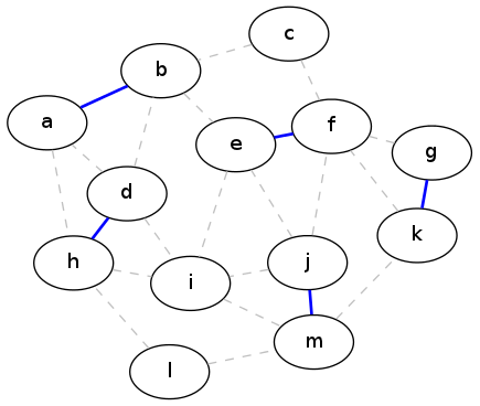
A greedy matching
Unfortunately, this is not an optimal solution. In fact, there is an example with only four vertices that demonstrates that the greedy strategy will produce sub-optimal solutions (can you come up with that example?). By contrast, here is an actual maximal matching for our running example graph:
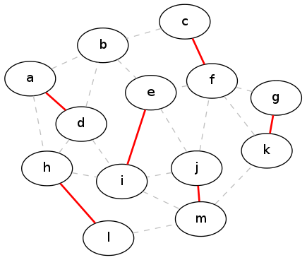
Optimal matching
The key shortcoming to the greedy strategy in this case is that never allows us to "change our minds" about a partial solution. The key to making greedy choices is that they can never be undone. The example above shows that we can end up with a case where the choices we have already made prevent us from adding any more edges to the graph, so we are "stuck" with a sub-optimal solution.
A sensible question to ask at this point is, how bad is the greedy solution? In the example above, the optimal solution has size six, whereas the greedy solution had size five. So is the greedy solution always at least one less than the size of the optimal? Or maybe five-sixths the size of the optimal? The next theorem answers these questions:
Theorem: Any matching produced by the greedy strategy has at least half as many edges as a maximum matching.
Proof: For the same graph G, consider a matching \(M_1\) produced by the greedy strategy, and a maximum matching \(M_2\). We want to compare the edges in each of these matchings.
First, remove all the edges that the two matchings have in common. Now consider the subgraph of G that results from combining the unique edges in \(M_1\) and \(M_2\). Call this combined graph \(G^*\). What does this graph look like?
One thing we know is that every edge in \(G^*\) has degree at most 2 — that is, there are at most two edges touching it. That's because if there were three edges, two of them would have to be in the same matching which is impossible.
Now because each vertex has degree at most two, this means that the graph \(G^*\) must just be a collection of simple paths and cycles. These are simply the only kind of things that you can get in a graph with maximum degree 2. Furthermore, the edges in these paths and cycles must be alternating between \(M_1\) and \(M_2\).
How long are the paths and cycles? They can't have length 1, because that would mean there's an edge which could have been added to one of the matchings without removing any of the other edges, but it wasn't added — a contradiction.
Finally, because the edges alternate, any path with length 2 has at most one more edge from \(M_2\) than from \(M_1\). Therefore the worst case comes with length-three paths, which will have twice as many edges from \(M_2\) as from \(M_1\). Since there may be arbitrarily many of these length-3 paths in \(G^*\), in the worst case \(M_2\) will have twice as many edges as \(M_1\). In other words, the maximal matching will never have more than twice as many edges as a greedy matching.
The following picture shows the two matchings (greedy and optimal) for the previous example, overlaid to show the graph \(G^*\) from the proof:
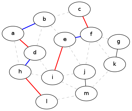
G-star graph
5.4 Speed-Correctness Tradeoff
Incidentally, there is an algorithm for the maximum matching problem that always finds solutions, and it's faster than the "brute-force" method of trying every possible subset of edges. The first algorithm to solve this problem in polynomial-time was invented by Jack Edmonds in 1965 and is called (appropriately) "Edmonds's algorithm", or sometimes "Edmonds's matching algorithm" to distinguish it from his other results. You can read the original paper here if you like. It's based on starting with the greedy algorithm and them improving it by finding certain alternating-color paths and loops, like in the proof above.
You might recognize the name Edmonds from a few units ago: he's the guy who (along with Cobham) proposed that every "tractable" algorithm must be polynomial-time. That is, its cost must be bounded by \(O(n^k)\) for some constant k, and where n is the total size of the inputs. Well section 2 of that paper on matchings is exactly where Edmonds made this claim, in the context of matching algorithms!
Part of the reason that Edmonds felt the need to talk about what is meant by a "tractable" algorithm is that his algorithm for finding maximum matchings is pretty slow: the worst-case cost is \(\Theta(n^4)\). This is polynomial-time, but the growth rate is faster than most other algorithms we have studied.
Although faster algorithms for this problem have been developed since then, none of them is as fast as the greedy algorithm above, which has worst-case cost \(\Theta(n+m)\) if the adjacency lists representation is used. So we have here the first example of a problem where correctness (or more properly, optimality) can be traded off against other resources such as time and space. Depending on the specific circumstances, a sub-optimal solution might be acceptable if we can get it really quickly. Or maybe we want to spend the extra time and get the best possible answer. The point is that there is a balance of concerns to account for, and not a single "best" algorithm.
6 Vertex Cover
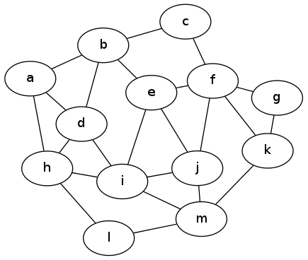
Consider the following scenario: You have a bunch of locations (vertices) that are connected by some waterways (edges). Your task is to choose which locations to use as bases, so that every waterway is touched by at least one base. That is, you want to choose a subset of the vertices so that every edge is adjacent to a vertex in the subset.
This problem is called vertex cover, and the optimization question is to find the smallest such subset, the minimal vertex cover. For example, have a look at this graph (same one we used for matching):
Vertex Cover Example
Here are some vertex covers for this graph:
{b, c, d, f, g, h, i, j, l}
{a, c, d, e, g, i, j, l, m}
{a, b, d, e, f, g, h, j, k, m}
{a, b, d, f, i, j, k, l}
{a, b, e, f, h, i, k, m}
{b, d, f, h, i, j, k, m}
Now we know that the first three can't be minimal vertex covers. What about the last 3, with 8 vertices each? They're the smallest we've found so far, but so what? Can you see any way of confirming that 8 is the smallest vertex cover without having to manually check every possible one?
6.1 Vertex Covers and Matchings
There is a deep and very important connection between vertex covers and maximal matchings in the same graph. We didn't define "maximal matching" before, but it means any matching that can't be trivially added to. (Notice that it is definitely not the same as a maximum matching!) For example, the greedy algorithm for matchings always outputs a maximal matching, but not necessarily a maximum one.
The following two lemmas relate the size of maximal matchings and vertex covers.
Lemma: Every vertex cover is at least as large as any matching in the same graph.
Proof: For each edge in the matching, one of its two endpoints must be in the vertex cover, or else it's not a vertex cover. But since it's a matching, none of the endpoints of any of the edges in the matching are the same.
In other words, just to cover the edges in the matching itself, the size of the vertex cover must be at least the size of the matching. Since the matching is part of the original graph, all those edges must be covered, and we get the stated inequality. QED.
For the example above, we know from before that the maximum matching in this graph has 6 edges. Therefore, from the lemma, every vertex cover must have at least 6 vertices in it. Unfortunately, this isn't quite enough to show that 8 vertices constitute a minimal vertex cover.
The next lemma gives an inequality in the other direction, to intracately tie these two problems together.
Lemma: The minimum vertex cover is at most twice as large as any maximal matching in the same graph. (Note maxiMAL, not maxiMUM.)
Proof: Let \(G=(V,E)\) be any unweighted, undirected graph. Take any maximal matching M in G. Now let \(C \subseteq V\) be a set of vertices consisting of every endpoint of every edge in M. I claim that C is a vertex cover.
To prove the claim that C is a vertex cover, suppose by way of contradition that it isn't. This means that there's some edge in E that doesn't touch any vertex in C. But this means that this edge doesn't touch any edge in M, and therefore it could be added to M to produce a larger matching. This contradicts the statement that M is a maximal matching. So the original assumption must be false; namely, C is a vertex cover.
From the way C was defined, its size is two times the size of M. Since the minimum vertex cover must be no larger than C, the statement of the lemma holds in every case. QED.
Combining these two statements, we see that any maximal matching M in a graph provides an upper and a lower bound on the size of the minimum vertex cover c:
\[|M| \le c \le 2|M|\]
Moreover, the second lemma is constructive, meaning that it doesn't just give us a bound on the size of the vertex cover, it actually tells us how to find one. Let's examine that algorithm more carefully.
6.2 Approximating VC
Here's the algorithm to approximate vertex cover, using the greedy algorithm for finding a maximal matching, and the construction described in the second lemma above:
def approxVC(G):
    C = set() # makes an empty set
    for (u,v,w) in G.edges():
        if u not in C and v not in C:
            C.add(u)
            C.add(v)
    return C
This algorithm is basically just finding a greedy matching and adding both vertices of every edge in the matching to the vertex cover. Unfortunately this doesn't always give the exact minimum vertex cover. But how close is it? The lemmas above provide the answer.
Theorem:
approxVC(G)always finds a vertex cover that is at most twice as large as the minimum vertex cover.Proof: From the second lemma, we know that the set C returned by the algorithm is always a vertex cover of G, and the size of C is \(2|M|\), where M is the greedy matching that is being found. But from the first lemma, we also know that any vertex cover must be at least as large as M. Therefore C is at most twice as large as the minimum vertex cover.
We therefore say that approxVC has an approximation ratio of 2 for the minimum vertex cover problem. We also saw a similar result earlier for the matching problem itself: the greedy matching algorithm returns a matching that is at at least one-half the size of the optimal maximum matching.
So we have a factor-two approximation algorithm for vertex cover, that uses a factor-two approximation algorithm for maximal matching. Now we know that there is a polynomial-time algorithm that always finds an optimal maximum matching — can we plug this into the VC approximation algorithm to solve this one in polynomial-time too?
The answer, which might be shocking, is a resounding no! These two optimization problems are optimizing in opposite directions: minimum vertex cover versus maximum matching. Therefore the very best matching algorithm will not give the best vertex cover. To approximate VC most effectively, we want a matching that is maximal (can't be added to), but which is not maximum. And the greedy matching algorithm provides this exactly! So the irony is that our sub-optimal matching algorithm which is fastest (the greedy one) gives the best approximation for vertex cover!
Now we are still left with the question of whether we can actually find the minimum vertex cover exactly, in polynomial-time. Can you think of any algorithm? If you do, please let me know, because there a 1-million dollar prize that we could split. But more on that in the next unit...