1 Shorted path in weighted graphs

BFS works great at finding shortest paths if we assume that all edges are equal, because it minimizes the number of “hops” from the starting point to any destination. But in a weighted graph, we care about the total sum of the weights along any candidate path, and want to miminize that value rather than the number of hops. In other words, it’s OK to take more turns in your driving directions, as long as the total time is less.

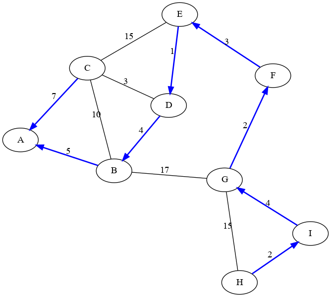
Consider the following graph. Here, the vertices may be intersections, and the edges may be roads, with expected time to travel as the weights.

Let’s consider the problem of finding the fastest route from vertex A to vertex H. A BFS would find us a path with the minimum number of hops, perhaps A - B - G - H. This path “looks” shortest, but it has total length \(5+17+15 = 37\) in the graph. There is definitely a shorter way!

We’ve already seen that the key difference between BFS and DFS is whether you store your fringe in a stack or queue. Dijkstra’s is also very similar, but uses a priority queue, which removes vertices according to which one has the shortest path from the starting vertex. Since we want the path with smallest weight, we will have a minimum priority queue.

2 Minimum Priority Queue

When we previously learned about priority queues and heaps, we focused on maximum priority queues, which are more useful for some applications such as HeapSort.

For graph algorithms, minimum PQ’s tend to be more useful. But the concept is exactly the same! If we use a heap to implement the min-PQ, then the smallest element will be at the top of the heap (a.k.a. the beginning of the array), and each heap node priority will be greater than or equal to the priority of its parent node. Instead of peekMax() and removeMax() we will have operations peekMin() and removeMin().

In fact, most programming languages and libraries only include a minimum priority queue, because changing between a min-PQ and a max-PQ just means changing the ordering of elements. In Java for example, you can select which kind of priority queue you want by changing how the compareTo() method works in your class, or by passing a Comparator to a certain constructor of the PriorityQueue() class.

2.1 Keyed priority queue

So far our priority queues have only had elements inserted, where the elements themselves were ordered in min-PQ or max-PQ order, and the entire element is what gets inserted, removed, or peeked at.

For some applications (including what we need for Dijkstra’s algorithm), we need not only the priority but also some associated key for each element. We could represent this with some simple class in Java such as:

class KeyPri<P extends Comparable<P>, K> implements Comparable<KeyPri<P,K> {
  private K key;
  private P priority;

  public KeyPri(K key, P priority) {
    this.key = key;
    this.priority = priority;
  }

  @Override
  public int compareTo(KeyPri<K,P> other) {
    return priority.compareTo(other.priority);
  }

  public K getKey() { return key; }

  public P getPriority() { return priority; }
  public void setPriority(newPriority) { priority = newPriority; }
}

Notice that it’s ordered by the priority, not the key — that way, any min-heap implementation will work out of the box. (Or, if all you have is a max-heap, you could negate the return value from compareTo() and use that just as well!)

In a keyed priority queue, we can also support two additional operations:

getPriority(key) -> priority
decreasePriority(key, newPriority)

What these methods do should be fairly obvious from the names. Note that we assume these methods will be called only for keys that are actually in the priority queue (otherwise an exception is raised), and for decreasePriority, the newPriority must be smaller or equal to the existing priority.

We also modify the add() method so that it takes two elements (key and priority), and modify peekMin() and removeMin() so they return a pair of key and priority. (In Java, these should return an instance of something class like KeyPri above.)

Note, in some textbooks the decreasePriority operation is called decreaseKey. We like the name decreasePriority better because it makes it clear there are two different things: the key is used only to lookup which element to change, and the priority that determines the PQ ordering is what actually gets updated. Just making you aware in case you read something about decreaseKey online or elsewhere — it’s talking about this operation!

2.2 Implementing getPriority and decreasePriority

Here’s an example of how a correct implementation of a keyed priority queue should work:

pq.add("A", 5); // key is A and priority is 5
pq.add("B", 3);
pq.getPriority("A"); // returns 5
pq.decreasePriority("A", 1);
pq.getPriority("A"); // returns 1
pq.removeMin(); // returns the pair KeyPri("A",1)
pq.removeMin(); // returns the pair KeyPri("B",3)
pq.removeMin(); // ERROR - the priority queue is now empty

Now let’s think about how to implement these two new operations. For this discussion, we will only consider priority queues implemented using arrays, since those are the most efficient ones we know of. The priority queue is organized by priority, and has no way to search by key — for that, we need to add an additional data structure of a Map associating each key to the index of that element in the array-based priority queue. If we implement the map with a hash table, getting and updating the indices in this array will be constant-time on average.

As is often the case, this extra data structure (the map associating each key with its index in the array) also requires extra “bookkeeping” to keep it up to date. Namely, every time any element changes indexes, for example in each step of a bubble-up or bubble-down operation, we also have to update the corresponding entry in the map. But again, if we use a hashtable, this is (average) constant time.

This means that the big-O running time of existing operations (add(), peekMin(), removeMin()) won’t change, and the running time of getPriority() will be \(O(1)\) on average, since it’s one hashtable lookup and then going to that index in the array.

The running time of decreasePriority() depends on which array-based priority queue data structure we use:

• Unsorted Array: Find the element in the array (\(O(1)\) using a HashMap), and update its priority (\(O(1)\), because it doesn’t have to move in the array). Total: \(O(1)\).

• Sorted Array: Find the element in the array (\(O(1)\) due to the HashMap), update its priority, and move it to the correct location in the array (\(O(n)\) due to the shifting). Total: \(O(n)\).

• Heap: Find the element in the array (\(O(1)\)), update its priority, and bubble it up (\(O(\log(n))\)). Total: \(O(\log(n))\). Notice, we know it a bubble-up because we are only decreasing the priority and it’s a minimum priority queue.

3 Dijkstra’s Algorithm

We are now ready to present the algorithm to find the shortest path between two points in a weighted graph. It is named after its inventor Edsger Dikstra, who was an early pioneer for the idea of computer science itself as a discipline, and who (among other honors) was one of the earliest recipients of the Turing award.

Dijkstra’s algorithm is the analog of breadth-first search for weighted graphs, where we use a keyed priority queue instead of a plain FIFO queue.

In BFS, there was never a scenario when a vertex’s parent would change. In Dijkstra’s, there is — the vertex gets a parent when it’s first adjacent to something, but that doesn’t guarantee that we won’t find a shorter path to it later, necessitating a change in parent. So we now have a threefold status for each node: either undiscovered (not yet seen at all), discovered (we’ve found one path bot not necessarily the shortest path), and visited (shortest path found and parent is now fixed).

Here is the pseudocode for Dijkstra’s algorithm:

dijkstras(G, start, end):
    fringe = empty keyed minimum priority queue
    parents = map from vertex label to another vertex label
    status = map from vertex label to one of two constants, DISCOVERED or VISITED
    fringe.add(start, 0)
    while fringe is not empty:
        cur, curDist = fringe.removeMin()
        # curDist is the shortest path length from start to cur
        status.set(cur, VISITED)
        if cur == end:
            # shortest path length is curDist
            # we could recover the shortest path using the parents map
            return
        for (v, w) in G.neighbors(current):
            # each element (v, w) in neighbors is a weight-w edge from current to v
            vdist = curDist + w
            if not status.containsKey(v):
                # found the first path from start to v
                status.set(v, DISCOVERED)
                parents.set(v, cur)
                fringe.add(v, vDist)
            else if status.get(v) == DISCOVERED and fringe.getPriority(v) > vDist:
                # found a shorter path from start to v
                parents.set(v, cur)
                fringe.decreaseKey(v, vDist)

3.1 Example run

OK, let’s get back to our example from above, and run Dijkstra’s algorithm to find the shortest path from A to G. Here’s a link to the picture of the graph in case you want to open it in a new tab or print it out so you can follow along.

To run through this example, we’ll look at the “state” of our three data structures status, parents, and fringe, at each step along the way. Here’s the initial state:

status:
parents:
fringe: (A, 0)

1. Remove (A,0) from the fringe.

   We mark vertex A as visited.

   Then we add 2 new fringe entries for each of A’s neighbors.

   status: A->VISITED, B->DISCOVERED, C->DISCOVERED
   parents: B->A, C->A
   fringe: (B,5), (C,7)

2. Remove (B,5) from the fringe.

   Vertex B is visited. G and D are added to the fringe. A is visited, so it’s ignored. For C, \(5+10>7\), so it’s left alone. G is now discovered, but we’re not done until our target vertex is visited, so we keep going.

   status: A->VISITED, B->VISITED, C->DISCOVERED, D->DISCOVERED, G->DISCOVERED
   parents: B->A, C->A, D->B, G->B
   fringe: (C,7), (D,9), (G,22)

   Notice: I’m not writing the fringe in order. It’s a minimum priority queue, so things will be removed according to the shortest distance first; but the actual order will depend on what data structure gets used, e.g., a heap.

   Also notice: The priorities stored in the fringe are the total distance the starting node to each discovered node, not just the weight of the last edge. Getting this wrong is a very common pitfall when implementing Dijkstra’s algorithm!

3. Remove (C,7) from the fringe.

   Vertex C is visited. A and B are visited already, so we ignore them. D is left alone because \(7+3>9\). E is added.

   status: A->VISITED, B->VISITED, C->VISITED, D->DISCOVERED, E->DISCOVERED, G->DISCOVERED
   parents: B->A, C->A, D->B, E->C, G->B
   fringe: (D,9), (G,22), (E,22)

4. Remove (D,9) from the fringe.

   Vertex D is visited. C and B are visited already, so they don’t change. E has a decreasePriority performed, and its parent changed, since \(9+1<22\).

   status: A->VISITED, B->VISITED, C->VISITED, D->VISITED, E->DISCOVERED, G->DISCOVERED
   parents: B->A, C->A, D->B, E->D, G->B
   fringe: (E,10), (G,22)

5. Remove (E,10) from the fringe.

   Vertex E is visited. Neighbors C and D are already visited. Neighbor F is added.

   status: A->VISITED, B->VISITED, C->VISITED, D->VISITED, E->VISITED, F->DISCOVERED, G->DISCOVERED
   parents: B->A, C->A, D->B, E->D, F->E, G->B
   fringe: (F,13), (G,22)

6. Remove (F,13) from the fringe

   Vertex F is visited. G has its parent changed and its priority decreased.

   status: A->VISITED, B->VISITED, C->VISITED, D->VISITED, E->VISITED, F->VISITED, G->DISCOVERED
   parents: B->A, C->A, D->B, E->D, F->E, G->F
   fringe: (G,15)

7. Remove (G,15) from the fringe. Since this is our target, once G becomes visited, we’re done.

We can now walk back the parent pointers: G-F-E-D-B-A. In reverse, this is the shortest path from the start (A) to the end (G), with total distance 15.

In fact, if we were to keep running, we would have found all of the shortest paths from A. The parent pointers encode a tree that gives the fastest path from A to any other node in the graph. Here they are drawn in blue:

4 Dijkstra’s Runtime

How long does Dijkstra’s take? Well, it’s going to depend on what data structures we use for the graph and for the priority queue. Let’s go through each of the costly steps in the algorithm:

• Calling removeMin():

  This will run \(n\) times, on a priority queue that holds at most \(n\) things.

• Calling neighbors():

  This also happens \(n\) times, at most once for each vertex in the graph.

• Calling add() or decreasePriority() on the fringe:

  One of these two things could happen for every edge from every vertex, so \(m\) times total. This happens on a priority queue of \(n\) things.

So to figure out the running time for Dijkstra’s, we have to fill in the blanks in the following formula:

\[n\text{(cost of removeMin()+cost of neighbors())}+m(\text{(cost of add() + cost of decreasePriority())}\]

Most of the time, we assume we’re using an adjacency list with a Hashtable, and a heap. In this case, this becomes \(n\log n + m\log n\), which is what is usually given as the runtime of Dijkstra’s for those not being very careful. And actually if we think about it, we can assume \(m\ge n\) here, as any unconnected vertices will never be visited. So the cost simplifies to just \(O(m\log n)\).

As always, it’s more important that you are able to use the procedure above to decide the running time of Dijkstra’s algorithm for any combination of data structures, rather than memorizing the running time.

For example (and a very important example!) suppose our graph is stored using the adjacency matrix representation rather than an adjacency list. Using a heap for the priority queue as above, we get \(O(n^2 + m\log n)\), because the neighbors() method in an adjacency list is more expensive.

There is now a better way! Because neighbors() is \(O(n)\), we can “afford” to use a priority queue with a slower removeMin() operation, if it means add() and decreasePriority() will get faster. And an unsorted array will do just that — removeMin() is \(O(n)\) whereas the other operations are constant-time. Overall, this brings the running time down to \(O(n^2)\).

For a very “dense” matrix where the number of edges \(m\) is close to \(n^2\), this is actually better than using an adjacency list and a heap!

5 All-Pairs Shortest Paths

Consider the “sledding hill” problem: I have a map of Annapolis with the elevation difference of each road segment marked, and I want to find the path — starting and ending at any spot — that gives the greatest total elevation difference. In such a situation, Dijkstra’s algorithm has two shortcomings:

• Dijkstra’s only works with non-negative edge weights. If the weights of edges can be positive or negative (such as elevation changes), Dijkstra’s is no longer guaranteed to find the shortest path the first time it visits a node, and so cannot be used in such situations. (Of course, if there’s a negative cycle, that is, a cycle with a total negative cost, then “shortest path” is ill-defined; you can just go round and round forever!)

• Dijkstra’s only finds the shortest paths from a single starting point. If we are interested in the shortest paths that could startand end anywhere, we would have to run Dijkstra’s algorithm \(n\) times, starting at every possible position.

What we’re talking about here is called the All-Pairs Shortest Paths Problem: finding the shortest paths between every possible starting and ending point in the graph, in one shot. For now, we’ll just consider the slightly simpler problem of finding the lengths of all these shortest paths, like the height of the best sledding hill. (Later we’ll say how you could also get the paths themselves.)

First think about how we would store the output. There are \(n\) starting points and \(n\) ending points, so that means \(n^2\) shortest path lengths — let’s put ’em in a \(n\times n\) matrix! This “shortest paths matrix” will be similar to the adjacency matrix, except that instead of storing just single edges we have all the shortest paths.

Note, if we didn’t have negative edge weights, we can actually use Dijkstra’s algorithm to solve All-Pairs Shortest Paths; we just have to run Dijkstra’s separately \(n\) times, starting from each node. The total running time would be \(O(nm\log n)\) using adjacency lists + heap, or \(O(n^3)\) using adjacency matrix + unsorted array.

6 Floyd-Warshall

The algorithm that we are going to learn for this problem is called the Floyd-Warshall algorithm, which is named after 2 people but actually has at least four different claimants to that title. This algorithm starts with the adjacency matrix of a graph, which we will gradually turn into the shortest paths matrix. (If your graph is stored in an adjacency list, you would have to convert it to an adjacency matrix first.)

The idea of the algorithm is that, at step \(i\), we will have the lengths of all shortest paths whose intermediate stops only include the first \(i\) vertices. Initially, when \(i=0\), we have just the single-edge paths (with no intermediate stops), and at the end when \(i=n\) we will have the shortest paths with any number of intermediate stops. Cool!

To see how this works, let’s go to an example:

We start with the adjacency matrix for this graph, where we put \(0\) as the distance from any node to itself and \(\infty\) as the distance between two nodes where no edge exists.

\[ \begin{array}{c|c|c|c|c|c|} & A & B &C &D &E &F \\ \hline A &0 &\infty &1 &\infty &\infty &2 \\ \hline B &\infty &0 &6 & \infty &1 & 2 \\ \hline C & 1 & 6 & 0 & 6 & 5 & 4 \\ \hline D & \infty & \infty & 6 & 0 & 2 & \infty \\ \hline E & \infty & 1 & 5 & 2 & 0 & \infty \\ \hline F & 2 & 2 & 4 & \infty & \infty & 0 \\ \hline \end{array} \]

This is essentially all the shortest path if no intermediate locations are allowed. The first thing to do, is allow node A to be an intermediate vertex in any of these paths. As you can see, that’s only going to (possibly) affect the shortest path from C to F. In deciding whether it does, we consider two options: the current shortest path from C to F (length 4), or the sum of the paths to C to A (length 1) plus the path from A to F (length 2). In this case, the sum is smaller, so that entry will be updated.

This update process can be described in pseudocode as follows:

updateShortest(Matrix, Source, Dest, NewStop):
    current = Matrix[Source][Dest]
    newPossibility = Matrix[Source][NewStop] + Matrix[NewStop][Dest]
    if newPossibility < current then
        Matrix[Source][Dest] = newPossibility

In this example, the path from C to F (and F to C, since the graph is undirected) gets improved to length 3:

\[ \begin{array}{c|c|c|c|c|c|} & A & B & C & D & E & F \\ \hline A & 0 & \infty & 1 & \infty & \infty & 2 \\ \hline B & \infty & 0 & 6 & \infty & 1 & 2 \\ \hline C & 1 & 6 & 0 & 6 & 5 & \color{red}3 \\ \hline D & \infty & \infty & 6 & 0 & 2 & \infty \\ \hline E & \infty & 1 & 5 & 2 & 0 & \infty \\ \hline F & 2 & 2 & \color{red}3 & \infty & \infty & 0 \\ \hline \end{array} \]

Next, we let B be an intermediate point in any path. What this means is that we run the updateShortest function on every possible starting/ending point combination in the matrix, looking for anywhere where stopping at B gives a shorter path. Once again, only a single path actually gets update here (E to F). But notice that this time we do better than just finding a slightly better path, B connects two vertices that otherwise would not be reachable, making the “shortest path length” go from infinity down to 3:

\[ \begin{array}{c|c|c|c|c|c|} & A & B & C & D & E & F \\ \hline A & 0 & \infty & 1 & \infty & \infty & 2 \\ \hline B & \infty & 0 & 6 & \infty & 1 & 2 \\ \hline C & 1 & 6 & 0 & 6 & 5 & 3 \\ \hline D & \infty & \infty & 6 & 0 & 2 & \infty \\ \hline E & \infty & 1 & 5 & 2 & 0 & \color{red}3 \\ \hline F & 2 & 2 & 3 & \infty & \color{red}3 & 0 \\ \hline \end{array} \]

The next “intermediate vertex” allowed is C. This time, we get a whole bunch of updates throughout the matrix (changes shown in red):

\[ \begin{array}{c|c|c|c|c|c|} & A & B & C & D & E & F \\ \hline A & 0 & \color{red}7 & 1 & \color{red}7 & \color{red}6 & 2 \\ \hline B & \color{red}7 & 0 & 6 & \color{red}{12} & 1 & 2 \\ \hline C & 1 & 6 & 0 & 6 & 5 & 3 \\ \hline D & \color{red}7 & \color{red}{12} & 6 & 0 & 2 & \color{red}9 \\ \hline E & \color{red}6 & 1 & 5 & 2 & 0 & 3 \\ \hline F & 2 & 2 & 3 & \color{red}9 & 3 & 0 \\ \hline \end{array} \]

Notice that one of the updated paths (D to F) used the first update (faster path from C to F) as part of its own shortest path, to get a length-9 path from D to F that goes through C and through A.

The next step is to update paths to allow the next vertex, D. But if you did this, you’d notice that none of the paths actually get updated. That’s okay! We move on to the next intermediate vertex, E. Two paths get shorter by going through E:

\[ \begin{array}{c|c|c|c|c|c|} & A & B & C & D & E & F \\ \hline A & 0 & 7 & 1 & 7 & 6 & 2 \\ \hline B & 7 & 0 & 6 & \color{red}3 & 1 & 2 \\ \hline C & 1 & 6 & 0 & 6 & 5 & 3 \\ \hline D & 7 & \color{red}3 & 6 & 0 & 2 & \color{red}5 \\ \hline E & 6 & 1 & 5 & 2 & 0 & 3 \\ \hline F & 2 & 2 & 3 & \color{red}5 & 3 & 0 \\ \hline \end{array} \]

Finally, we shorten three paths by allowing them to go through the last node, F:

\[ \begin{array}{c|c|c|c|c|c|} & A & B & C & D & E & F \\ \hline A & 0 & \color{red}4 & 1 & 7 & \color{red}5 & 2 \\ \hline B & \color{red}4 & 0 & \color{red}5 & 3 & 1 & 2 \\ \hline C & 1 & \color{red}5 & 0 & 6 & 5 & 3 \\ \hline D & 7 & 3 & 6 & 0 & 2 & 5 \\ \hline E & \color{red}5 & 1 & 5 & 2 & 0 & 3 \\ \hline F & 2 & 2 & 3 & 5 & 3 & 0 \\ \hline \end{array} \]

Now this matrix stores the shortest path lengths between any pair of vertices in the original graph. Check it if you don’t believe me!

The only detail we’ve glossed over is how you would actually recover these shortest paths. The answer is that you have parent pointers, just like we did for Dijkstra’s algortihm. Except, instead of just storing \(n\) parent pointers indicating how to get back to the single starting point, we will need to store \(n^2\) parent pointers for how to get back from any point to any possible starting point, in the shortest way! Naturally, we would use another matrix to store such pointers.

The pseudocode for Floyd-Warshall looks like this:

FloydWarshall(G):
    Matrix = copy of Gs adjacency matrix
    for each Intermediate in G.vertices():
        for each Start in G.vertices():
            for each End in G.vertices():
                updateShortest(Matrix, Start, End, Intermediate)

This shows the real power of Floyd-Warshall’s algorithm: its simplicity. It’s just three nested for loops! \(O(n^3)\) running time.