This is the archived version of this course from the Spring 2013 semester. You might find something more recent by visitning my teaching page.
Readings:
- MR, Sections 2.1 and 10.3
Remember at the beginning of the course we said that most randomized algorithms are either simpler or faster than the deterministic version (or both). In the last unit on data structures, we saw some randomized solutions that had the same asymptotic speed as things like AVL trees and red-black trees, but which are much simpler to program.
This unit is about the other end. We will look at two important algorithms for which the randomized solution is faster than any deterministic algorithm. These algorithms are not necessarily going to be simple, but they do give an improvement over the worst-case deterministic cost. They demonstrate that randomness actually has some "power" to it; it isn't just a tool to let us be lazy programmers.
Beginning of Class 14
1 Game Tree Evaluation
1.1 Game trees
Consider a 2-person game like chess, checkers, tic-tac-toe, and so on, which has the following basic properties:
- Players take turns moving
- Both players can see the whole board; there are no secrets
- Players have complete control over the outcome of the game; there is no dice rolling or chance element
- The outcome is either win or lose. Whenever one player wins, the other one loses.
Some adjectives you might see to describe this kind of game are perfect-knowledge, zero-sum, sequential, discrete, and non-stochastic. You don't have to worry too much about these terms (they come from game theory); just make sure your game follows the rules listed above and it will work for what we're doing here.
And what is it that we're doing? Well, we want to model, understand, and ultimately devise winning strategies for these kind of games. In order to do that,
A game tree is a graph used to represent a two-person game. Here are the basic properties:
- Each node in the graph represents a partial configuration of the game. In board games like tic-tac-toe or checkers, a partial configuration is just a game board with an arrangement of pieces or marks on it.
- The root node of the graph is the starting configuration. In tic-tac-toe, this is just an empty 3 by 3 grid.
- Every edge (a.k.a. branch or connection) in the tree represents a single player's move on their turn. In tic-tac-toe, each edge corresponds to one player putting their X or their O in one position of the grid.
- Each leaf node is a "terminal configuration", meaning that no further moves are possible. Each leaf node represents a win or a loss, which can be explicitly determined. That's important, so I wrote it in bold. See?
In class we drew some examples of game trees. The internet has many more, so I'm not going to draw one out here.
So far we know that each leaf node is classified as either a win or a loss. But what about the other nodes? What's the point? We're going to use game trees to determine whether a game is always winnable by some player. That is, is there a strategy of moves that the player can employ to guarantee themselves a win, every time? Evaluating a game tree gives us this answer!
For what follows, I'm going to use the first person ("I", "me") to talk about the player whose winning strategy we're trying to determine.
The way it works is, the non-leaf nodes in the tree (a.k.a. "internal nodes") are classified as OR nodes or AND nodes. An OR node is evaluated as a win if and only if at least one of its child nodes evaluates to a win. This corresponds of course to the boolean "or" operator, and in terms of a game it means a move that I make, where I can choose which move it is. If there is at least one move I can make that still guarantees me a win, then I can always win - simple as that!
An AND node is evaluated as a win if and only if every one of its child nodes evaluates to a win. In the game, this corresponds to the other player's turn: if I can guarantee a win no matter what move the other player makes, then I can always guarantee a win.
Putting this together, evaluating a game tree just means working up from the leaves to the root, computing ANDs and ORs of the nodes, until we get to the root. The nodes on each level of the tree will alternate between AND and OR nodes, since we are talking about 2-player games where the players alternate taking turns. If the root node is OR, then "I" am going first, otherwise I am going second. If the result at the root is "win", then there is a winning strategy that will guarantee I can never lose!
About ties: Most of the 2-person games we are talking about are not really win-loss games; there can also be ties. But our definition of game trees doesn't allow for that.
Beginning of Class 15
1.2 Deterministic Algorithm
We're going to try and make the fastest possible algorithm for evaluating a game tree. For these algorithms, assume that any subtree of a game tree (including the entire tree itself) is represented by a node u with the following properties:
u.leafis true or false depending on whether this node has no children.u.op, for a non-leaf node, is eitherANDorORto indicate the operation at that nodeu.win, for a leaf node, is true or false depending on whether this configuration represents a "win" or "lose" outcome.u.children, for a non-leaf node, iterates through each child in left-to-right order.
Now that we have the terminology down, we can consider a basic deterministic algorithm:
def gt_eval_0(u):
    '''Returns true if this node evaluates to a win, otherwise false'''
    if u.leaf:
        return u.win
    elif u.op == 'OR':
        result = False
        for child in u.children:
            result = result or gt_eval_0(child)
        return result
    elif u.op == 'AND':
        result = True
        for child in u.children:
            result = result and gt_eval_0(child)
        return result
This algorithm works fine, but it is rather slow. No matter what, it does recursive work at every single node in the tree. For a game tree with \(n\) nodes total, the cost of this algorithm is \(O(n)\).
Can we do better? Of course. The first optimization is rather easy to see - in fact, it's built-in to most programming languages! If you have a C++ line such as
return foo() && bar();
then the call to bar() will never even be evaluated if foo() returns false. That's because the value "false" and-ed with anything else will always produce false at the end, so there is no need to evaluate bar() in this case. This optimization is commonly called short-circuit evaluation, and it can be applied similarly to the "or" operation. We can speed up the deterministic algorithm above by incorporating this idea:
def gt_eval_determ(u):
    '''Returns true if this node evaluates to a win, otherwise false'''
    if u.leaf:
        return u.win
    elif u.op == 'OR':
        for child in u.children:
            if gt_eval_determ(child) == True:
                return True
        return False
    elif u.op == 'AND':
        for child in u.children:
            if gt_eval_determ(child) == False:
                return False
        return True
This algorithm certainly has the potential to be faster than gt_eval_0, because it will "short-circuit" the evaluation whenever possible. But will it actually be faster? Unfortunately, the answer is no, at least not in the worst case. For example, here's a worst-case tree with branching factor \(k=2\) and height 3:
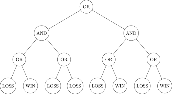
Worst-Case Game Tree
You can confirm that the algorithm above is "forced" to evaluate every single node in this tree, recursively. The overall output is "true" (a WIN is always possible for the first player), but \(O(n)\) work must be done to obtain this answer.
In fact, it is not too difficult to see that any deterministic algorithm could be forced to do this much work in the worst case. The way the proof works is like this: take any deterministic algorithm, and imagine an "adversary" that will construct the worst-case for that algorithm. The worst-case will look just like the example above, except that it is constructed dynamically by the "adversary", as the algorithm asks questions about whether each leaf is a win or a loss. We saw an example of this in class.
In other words, no matter how clever we make a deterministic algorithm with tricks like the "short circuiting" above, their cost will always be \(O(n)\) in the worst case. The short-circuiting doesn't really help.
1.3 Randomized Algorithm
By now you should know what's coming - randomization! The randomized version of the game tree evaluation algorithm is really straightforward. It's exactly the same as the short-circuited version, except that the order in which child nodes are evaluated is chosen randomly instead of always going left-to-right. Here's pseudocode:
def gt_eval_rand(u):
    '''Returns true if this node evaluates to a win, otherwise false'''
    if u.leaf:
        return u.win
    elif u.op == 'OR':
        for child in random_order(u.children):
            if gt_eval_rand(child) == True:
                return True
        return False
    elif u.op == 'AND':
        for child in random_order(u.children):
            if gt_eval_rand(child) == False:
                return False
        return True
Importantly, this random order is the "sampling without replacement kind" - otherwise we might keep picking and re-evaluating the same child over and over again!
This randomization is straightforward enough, but will it really help? Certainly the worst-case will still be \(O(n)\) nodes evaluated. In fact, this seems inevitable at first. If the root of the tree is "OR" and the game is not winnable, then every child will have to be evaluated recursively in the inner for loop, no matter what the order is! Similarly if the root is "AND" and the game is winnable; every child gets recursively evaluated, no matter what the order.
The trick to this analysis is looking down two levels into the recursion. Consider the unlucky case described above: the root node operation is "OR" and the ultimate return value is False. Then every subtree of the root must be recursively evaluated. In fact, we know more than this: each of these subtrees will be an "AND" node that evaluates to False. And this means that, while the top-level "OR" node is not short-circuitable, each of its subtrees is short-circuitable. The opposite is true when the root node is "AND" - either this node is short-circuitable, or all of its subtrees are.
Now we are ready to start writing down some recurrences to do the analysis. For this analysis, we will assume the branching factor is \(k=2\); that is, every node has exactly two children. You will consider other branching factors in the problems.
As we have seen above, there are two cases to consider, depending on whether the root node is short-circuitable or not. So define \(T(n)\) to be the expected cost of randomized game tree evaluation on a size-n tree that is not short-circuitable, and define \(S(n)\) to be the expected cost when the root node is short-circuitable. The base case for both of these is
\[T(1) = S(1) = 1\]
The recursive case for \(T(n)\) is easier so we'll write that down first:
\[T(n) = 1 + 2S(\frac{n}{2}),\quad n\ge 2\]
This is because, when the tree is not short-circuitable, the randomized algorithm always requires both recursive calls, but those subtrees will both be short-circuitable.
The recursive case for \(S(n)\) is where the randomization comes in. The number of recursive calls could be 1 or 2. It is 1 if the algorithm is lucky and chooses the short-circuiting subtree first. Otherwise, if the algorithm is unlucky, it might choose the wrong order and still do 2 recursive calls. And in the worst case, all of these recursive calls will be on subtrees that are not short-circuitable. This leads to the equation
\[S(n) = \frac{1}{2}\left(1 + T(\frac{n}{2})\right) + \frac{1}{2}\left(1 + 2T(\frac{n}{2})\right)\]
which simplifies to
\[S(n) = 1 + \frac{3}{2}T(\frac{n}{2})\]
Now substitute this into the equation above and we get a recurrence for the whole thing:
\[T(n) = 1 + 2\left(1 + \frac{3}{2}T(\frac{n}{4})\right) = 3 + 3 T(\frac{n}{4})\]
This is a now a simple, standard-looking recurrence that can be solved by a variety of methods, for example the so-called "Master Method" from Algorithms class. Solving the recurrence "manually" by expanding also works:
\[T(n) = 1 + 3 T(\frac{n}{4}) = 2 + 9 T(\frac{n}{16}) = 3 + 27 T(\frac{n}{64}) = \cdots = k + 3^k T(\frac{n}{4^k}) \]
Setting \(k=\log_4 n\) will bring it to the base case:
\[T(n) = \log_4 n + 3^{\log_4 n}T(1) = \Theta(n^{\log_4 3}) \approx \Theta(n^{0.792}) \]
Therefore our randomized algorithm is a significant improvement over the deterministic \(O(n)\) algorithm. But it's even more important than that, because we proved that any deterministic algorithm for game tree evaluation will have worst-case cost \(O(n)\). So this problem is similar to the "airplane terrorists" scenario in that it really shows the power of randomization to do something faster than would be possible without it.
Beginning of Class 16
2 Minimum Spanning Tree
Supplemental reading:
- Minimum spanning trees (Wikipedia)
- Kruskal's algorithm (Wikipedia)
- Boruvka's algorithm (Wikipedia)
- Original paper for Karger-Klein-Tarjan (Journal of the ACM)
- Easier analysis of Karger-Klein-Tarjan by Timothy Chan (click the "PDF" link at the top-left corner)
Imagine you run a telecommunications company and are trying to run a new high-speed fiber optic cable to a number of locations in the area. You want to connect all of them using the least amount of cabling possible, or at the lowest cost, whatever. We don't care how the locations get connected, just that they are all connected.
This problem can be modeled using a graph: The nodes of the graph are the locations, and the edges between nodes have the cost of laying fiber optic cable between those two locations. And now the telecommunications company's predicament is asking for a collection of edges (connections) in this graph that connects all the nodes, and has the least possible weight. This is called a minimum spanning tree or MST.
You learned about some MST algorithms in IC 312 (Data Structures). These might have included Kruskal's algorithm or Prim's algorithm, or possibly Boruvka's algorithm. These algorithms are all interesting and worth understanding, and (importantly) they all cost \(O((n+m)\log n)\) time in the worst case to find a minimum spanning tree of a graph with \(n\) nodes and \(v\) edges.
(Actually, there's an advanced data structure called a Fibonacci Heap that can be used to run Kruskal's algorithm in \(O((n+m)\alpha(n))\) time, where \(\alpha(n)\) is the inverse Ackermann function that grows extremely slowly.)
What this means is, in summary, there is no way to compute MSTs deterministically in linear time. Notice that "linear time" here means linear time in the size of the input, which is \(O(n+m)\). (We assume the graph is stored using an adjacency list.)
2.1 Boruvka Algorithm
Boruvka's algorithm is actually the oldest of the MST algorithms mentioned above, and it's also the basis for our randomized improvements. Unlike Kruskal's or Prim's algorithm, the way Boruvka's algorithm works is by a series of phases or Boruvka steps, each of which does a significant amount of work to compute the MST. Here's how a single Boruvka step works:
def BoruvkaStep(G):
    T = {} # empty set of edges
    for each node u in G:
        E = least weight edge touching node u
        add E to T
    contract all edges of T in G
    return T
A couple comments on this:
- Some edges might get added to
Tmore than once, butTonly has one copy of any given edge. - The edge "contraction" on the second to last step combines nodes joined by any edge in
Tinto a single node, but without removing any edges. So the resulting graph might have "multiple edges" (more than one edge between the same pair of nodes) or "loops" (an edge going from a node back to itself). - The returned set
Tcontains some, but not all, of the edges in the MST of G. However, any MST of the contracted graph, plus the edges inT, will form an MST of G.
How fast is a single Boruvka step? For each node, it has to go through all that node's edges once, to find the shortest edge attached to that node. Since every edge is adjacent to 2 nodes, a given edge is looked at at most twice in this process. So the total cost for finding all the edges for T is \(O(m+n)\). And in fact that's the cost of the whole thing: linear-time in the size of the graph.
To use Boruvka's algorithm to compute an entire MST requires multiple Boruvka steps, of course. How many? Well, each Boruvka step will reduce the number of nodes by at least a factor of 2. That is, the resulting contracted graph will have at most \(n/2\) nodes. This is because the for loop adds edges to T \(n\) times, and each edge can only be added two times, since it has only two endpoints. Contracting each edge reduces the number of nodes by one, so contracting \(n/2\) edges reduces the number of nodes to \(n/2\).
This means that, in order to compute the entire MST, you must do enough Boruvka steps until the number of nodes equals 1, which would be \(\log n\) steps. Hence the worst-case cost of Boruvka's algorithm is the same as the others, \(O((m+n)\log n)\).
Beginning of Class 17
2.2 MST Verification
Imagine being given a tree in a graph, that someone claims is the MST of that graph. How could you check whether they are telling the truth? This is known as the MST verification problem, and it turns out to be important in computing the MST itself!
The algorithm works on the following principle:
Fact: If \(T\) is an MST of \(G\), then for every edge \((u,v)\) in \(G\) that is not in \(T\), adding \((u,v)\) to \(T\) creates a cycle, and \((u,v)\) the the highest-weight edge in that cycle.
To verify whether \(T\) is an MST of \(G\), the algorithm splits all the edges of \(G\) into what are called "heavy" and "light" edges:
- An edge in \(G\) is T-heavy if adding it to \(T\) creates a cycle, and that edge has the largest weight along the cycle.
- Otherwise - if adding the edge doesn't create a cycle, or if it doesn't have the largest weight along that cycle - the edge is T-light.
Any T-heavy edge can't possibly be part of any MST of \(G\). Essentially, the tree \(T\) proves that these T-heavy edges are not part of the MST. This means that \(T\) is an MST if and only if every edge of \(G\) that is not in \(T\) is T-heavy. Hence, the verification succeeds if and only if the T-light edges are just the edges that are in \(T\) itself.
The important thing is that linear-time MST verification algorithms exist (we won't go into the full details though), and these algorithms will actually spit out a list of T-heavy and T-light edges. This is really useful, because even if \(T\) itself is not an MST of \(G\), we know for sure that the MST contains only T-light edges from \(G\). Given a candidate MST, this verification algorithm can spit out a (hopefully) small subset of edges from \(G\) to recursively search for the true MST.
2.3 Karger, Klein, and Tarjan (Randomized!)
In 1995, Karger, Klein, and Tarjan published a paper that revolutionized the MST world by showing how the old idea of Boruvka's algorithm could be combined with the idea of MST verification in order to do something no one else could: compute MSTs in linear time. The only caveat is that they had to use randomization to do it. Are you ready for the algorithm? Here it is:
Input: Graph \(G\) with \(n\) nodes and \(m\) edges
Output: A minimum spanning forest of \(G\). (A forest is a collection of trees; this MSF will be a collection of MSTs of all the connected components of \(G\).)
- Run a Boruvka step on \(G\) to shrink it down.
- Run a second Boruvka phase on the result from step (1).
- Run a third Boruvka phase on the result from step (2). Call this result after 3 Boruvkas \(G'\)
- Construct a random subgraph \(H\) of \(G'\), by randomly choosing each edge of \(G'\) to be in \(H\) with probability \(1/2\).
- Recursively call this MST algorithm on \(H\), returning \(F\), the minimum spanning forest of \(H\).
- Use a MST verification algorithm on \(F\) to compute all the \(F\)-light edges in the original \(G'\) from step (3). Construct a new graph \(G''\) which consists of the F-light edges from \(G'\).
- Recursively call this MST algorithm on \(G''\), returning \(T\) which is the MSF of \(G''\).
- Return \(T\). It's the MSF of \(G\) as well!
The cost of this algorithm is determined by the sizes of the two recursive calls on steps (5) and (7), on graphs \(H\) and \(G''\). In class, we saw that the sizes of these graphs are:
- \(H\) has at most \(n/8\) nodes and an expected number of \(m/2\) edges.
- \(G''\) has at most \(n/8\) nodes and an expected number of at most \(n/4\) edges.
This means the total size (nodes plus edges) of \(H\), plus the total size of \(G''\), is:
\[\frac{n}{8} + \frac{m}{2} + \frac{n}{8} + \frac{n}{4} = \frac{n+m}{2}\]
In other words, the total size \(s = m + n\) is decreasing by at least half, on average, at each recursive level. So the total cost of the algorithm is described by the recurrence
\(T(s) \le s + T(s/2)\)
which solves to \(T(s) \in O(s)\). Therefore the total worst-case cost of this randomized MST algorithm, in expectation, is \(O(m+n)\), linear-time in the size of the input. AMAZING! WORLD CHANGING! To this day, the only linear-time MST algorithm is this way, using randomization. Again, the power of random numbers is revealed. Observe that, in this case, the randomized algorithm is not simpler than the deterministic version, but it is "better" in the sense of asymptotic running time. This is different than the randomized algorithms and data structures we have seen before.