This is the archived version of this course from the Spring 2013 semester. You might find something more recent by visitning my teaching page.
Readings:
- MR, Sections 8.3, 8.2, and Appendix C
In this unit, we are going to look at some randomized data structures. We'll go into more detail on this later, but it is important to recognize up front what is random and what is not. In a randomized data structure, like any other data structure, the contents are not chosen randomly; they are picked by whoever is using the data structure. What is going to be random is the way those items are organized internally, the links and ordering of the user's input to facilitate efficient retrieval. We will see how choosing this structure randomly gives the same expected behavior as the more complicated data structures you've already learned about.
Beginning of Class 8
1 Expected Value and Probability
We saw expected value defined in Unit 1, and it's going to become more and more important as we go along. If you read in the textbook or on most online sources, you'll see a bunch of discussion about random variables. We'll try to avoid the formalisms and complictions to the extent possible here though.
Remember that expected value is, intuitively, just the average of some quantity weighted according to the probabilities of each quantity value occurring. Take lottery winnings as a simple example:
Consider a very simple lottery, where each ticket costs 1 dollar, there is one winner who gets J dollars, and the chances of winning are one in a million. We want to decide how large J needs to be before it's worth it to play. This will correspond to the expected value of the payoff. Here there are two possibilities: with probability \(\frac{999999}{1000000}\) we will lose 1 dollar, and with probability \(\frac{1}{1000000}\) we will win \(J-1\) dollars. Therefore the expected payoff is
\[\mathbb{E}[\text{winnings}] = \frac{999999}{1000000}(-1) + \frac{1}{1000000}(J-1) = J\cdot 10^{-6} - 1\]
You could solve this equation for an expected value of 0 to discover that, if the jackpot is worth at least a million dollars, we expect to gain money on average by playing.
OK, so in this simple example that's not so surprising. But the same idea holds more generally. For example, there might be some intermediate wins in the lottery with lower payoffs but higher probability, or we might account for the probability of a spit jackpot, etc. The point is that expected value is a useful tool to make decisions in the face of uncertainty, when we know the probabilities of each thing occurring.
Now here's a fact about expected value that we will need below:
Linearity of expectation
For any random values \(X_1, X_2, \ldots, X_n\),
\[\mathbb{E}[X_1 + X_2 + \ldots + X_n] = \mathbb{E}[X_1] + \mathbb{E}[X_2] + \cdots + \mathbb{E}[X_n]\]
In other words, the expected value of the sum of a bunch of things, is exactly the same as the sum of the expected values. This means that, if the expected value of my winnings after playing the lottery once is even as small as $0.01, then if I play 1000 times the expected winnings go up to $10. If I could afford to play a million times, well then the expected winnings go up substantially.
If this all seems way to obvious, consider (as we will) the expected value of the maximum. You might be tempted to say that \(\mathbb{E}[\max(X_1, X_2)] = \max(\mathbb{E}[X_1], \mathbb{E}[X_2])\). Not so! Consider the height of U.S. males. The average height of adult males is 5'10", or 60 inches. That means that the expected height of a single randomly-chosen adult male is exactly 60 inches.
But what if I choose 100 U.S. males randomly, and consider the maximum height among those 100? Since they all have the same expected height, the maximum expected height among them is exactly 60 inches. But would you actually expect the tallest among those 100 to be 60 inches? I think not. We would need more information to determine what the expected value of the maximum is precisely, but certainly it is greter than the maximum of the expected values. More on this later.
2 Skip Lists
Skip lists are given excellent coverage in your textbook and online, so I won't go into as much detail in this section of the notes. We'll just cover the highlights.
Consider a linked list. It's a wonderfully simple data structure, efficient in storage, blazingly fast to iterate through, and easy to implement. However, there's a big disadvantage: accessing the middle. In a normal linked list, there's no way to get to the middle of the list other than to go through half of the list, which is not very fast.
Hence the skip list. The idea is to start with a simple linked list (this will be "level 0"), and then build up more linked lists on top, each of which contains a subset of the nodes below it. So the higher-level linked lists "skip" over some items in the lower-level linked lists. Extending this idea up gives us a lot of the simplicity of linked lists, with the added ability to be able to quickly jump to any spot.
Oh, and one more thing: Skip lists are always ordered, and there are always two special values \(-\infty\) and \(+\infty\) at the ends. Now behold the skip list:
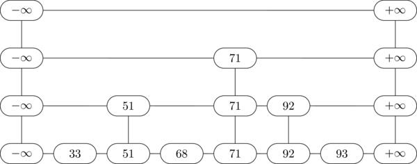
Example Skip List
Some terminology:
- This skip list six items and we write \(n=6\).
- The 6 keys are 33, 51, 68, 71, 92, and 93. There may be some values associated with each item as well, but we haven't drawn that because it doesn't affect the way the data structure works.
- Each item has a tower in the skip list, with varying heights. The height of the tower for 33 is 0, the height of the tower for 51 is 1, and the height of the tower for 71 is 2.
- The height of the skip list is the height of the infinity towers, which is one more than the height of the tallest item tower. The skip list above has height 3.
- The skip list consists of linked lists at different levels. In the example above, level 0 has all the items, level 1 has only 3, level 2 has just 71, and level 3 doesn't have anything in it. The hightest level in any skip list is always empty.
- Each tower consists of some number of nodes, according to the height of the tower. The total size of the skip list is simply the number of nodes in it. The example above has size 10 (not counting the infinity towers on the ends).
- In practice, the towers are usually stored as a single struct, with a list of forward links corresponding to the tower's height.
We usually use skip lists to implement the dictionary ADT, supporting the search, insert, and delete operations. We'll talk more about insert and delete later, but first let's cover how searching is performed in a skip list, since that's kind of the whole point!
Skip List Search
To search for key k in a skip list S, do the following:
- Start with v as the top-left most node in S
- If the node to the right of v has key less than k, then set v its neigbor to the right.
- Else if v is not at level 0, set v to the node below it.
- Else, we are done. Either the key of v is equal to k or k is not in S.
- Go back to step 2 and repeat until step 4 is triggered.
For example, to search for 80 in the skip list above, we start at the top-left infinity node, then move down to level 2, then right to 71 on level 2, then down to 71 on level 1, and finally down to 71 on level 0. Now the node following v has key larger than k (\(92 \gt 80\)), and we can't go down past level 0, so we conclude that 80 is not in this skip list.
Beginning of Class 9
3 Randomized Data Structures and Skip-Insert
To insert in a skip list, you first choose the height of the new node to be inserted, then insert it where it goes at each level up to that height.
You can see the details on the insertion part from my code in the problems. The interesting thing here is actually the height choosing algorithm:
def chooseHeight():
    h = 0
    while randomBit() != 1:
        h = h + 1
    return h
Pretty simple, huh? Basically, we randomly choose bits until we get a 1, and then the number of zeros that were chosen is the height of the new node that will be inserted.
Beginning of Class 10
4 Skip List Analysis
The question is, what is the expected height of a new node? Remember that expected height means each possible height gets multiplied by the probability of getting that height, then these are all added up to give the weighted sum. Here's the formula:
\[E[h] = \frac{1}{2}\cdot 0 + \frac{1}{4}\cdot 1 + \frac{1}{8}\cdot 2 + \cdots = \sum_{i=0}^\infty \frac{i}{2^{i+1}}\]
This is a pretty standard summation that appears on the much-beloved theoretical computer science cheat sheet and the sum comes to (drum roll..) 1. So the expected height of a skip-list node is 1.
We also showed in class how this does NOT imply the expected height of the entire skip list is 1. This is because the expected value of the maximum (maximum height of any item in the skip list) is NOT the same as the maximum expected value! In fact, the expected height of a skip list is \(O(\log n)\), which we went over in class.
To analyze the cost of search is a little more tricky. Basically, you do it backwards. Starting with the node that gets searched for, trace the search path backwards to the top-left node in the skip list. If we define \(T(h)\) as the expected length of a search path in a height-\(h\) skip list, we get the following recurrence:
\[T(n) \le \left\{ \begin{array}{ll} 0,& n=0 \\ 1 + T(h-1),& \text{if last leg is vertical}\\ 1 + T(h),& \text{if last leg is horizontal} \end{array} \right.\]
The big question is whether the last leg of the search is vertical or horizontal. Well, it just depends on whether the height of the last tower is greater than 0. But we know how the tower height was chosen - and the probability that it's greater than 0 is exactly \(\frac{1}{2}\). So the \(n\gt 0\) case of the recurrence becomes:
\[T(h) \le \frac{1}{2}(1 + T(h-1)) + \frac{1}{2}(1 + T(h))\]
Multiply both sides by 2 and subtract \(T(h)\) from both sides, and we get:
\[T(h) \le 2 + T(h-1)\]
which means \(T(h) \in \Theta(h)\). In other words, the expected cost of search is the same (up to a constant) as the expected height, which we already know is \(\Theta(\log n)\). This is the same as AVL trees! Hooray!
Beginning of Class 11
5 Random BSTs
- Great reference: notes by Conrado Martinez
A randomized binary search tree is just like a regular BST, except that we make random choices on insertion in order to keep it balanced. The way it works specifically is that, when we insert a new node into a tree that already has \(n-1\) nodes, the new node will become the root with probability exactly \(1/n\). In other words, every time a new node is inserted, there is a one out of (number of nodes in the tree) chance that it becomes the new root.
We went through a number of examples in the class. The key is that this algorithm for insertion gets applied recursively at every level down the tree. So when we insert a new node, it has a small probability of becoming the new root. But then it's recursively inserted into one of the two subtrees, and it has a less-small probability of being the root of that subtree. And so on down to the bottom.
Something really cool happens when we consider the probability that any element is the root of the final tree. Say we have the kth inserted item. It had probability \(\frac{1}{k}\) of being the root when it was inserted. Then in order for it to stay being the root, the next element must not have been chosen to be the root: this happens with probability \(\frac{k}{k+1}\). Then the next one must not have been the root either; the probability there is \(\frac{k+1}{k+2}\). Multiply all these out and you get the probability that the \(k\)th item is the root equals:
\[\frac{1}{k}\cdot \frac{k}{k+1} \cdot \frac{k+1}{k+2} \cdots \frac{n-1}{n} = \frac{1}{n}\]
So every single element has equal probability of being the root. Awesome! When you apply this recursively down the tree, you see that the expected height of the tree is \(\Theta(\log n)\). So this is a way of getting the same balance as an AVL tree or 2-3 tree, but by using randomness to do it instead of all those annoying tree rotations and extra complications.