Reading: CLRS, Chapter 17 (Mostly just 17.1 and 17.4).)
Beginning of Class 41
1 Amortized Analysis
You may remember the idea of amortized analysis from Data Structures class, when you looked at the problem of creating an extensible array, like the vector class in C++. As a reminder, the basic principle there was that a single array insertion might be expensive (if we have to allocate a new array), but the average cost over a whole sequence of insertions is small (constant-time).
Here's the formal definition:
Given a sequence of m consecutive operations, the amortized cost per operation is defined as the total cost of the whole sequence, divided by m.
Amortized analysis is useful in situations where the worst-case cost of some algorithm is expensive, but it's somehow impossible to have that worst-case cost occur many times in a row. Note the language like "in a row" or "consecutive operations" or "sequence" — this is really important! If we were just talking about the average cost of m randomly-chosen operations from all the possibilities, well that would be average-case analysis. Amortized analysis is something different — it's the worst case cost among all sequences of m operations.
This is why amortized analysis is an algorithm analysis tool that is usually applied to algorithms on data structures. The reason is that having a sequence of, say, searches, doesn't really have any special meaning if the searches are all on different arrays. But if we have a sequence of operations on the same data structure, like a bunch of searches on the same array, well there might be something to that...
2 Binary Counter
Let's start with a simple example of amortized analysis: incrementing a binary counter. Specifically, say we have a k-bit binary counter (so it can store any integer from 0 up to \(2^k-1\)), and we want to increase it from the current integer to the next integer, where we have to operate one bit at a time. Here's an algorithm to do that:
Binary counter increment
Input: Array D of 0's and 1's, of length k
Output: D is incremented to the next larger integer.
for i from 0 to k-1
  if D[i] = 0 then
    D[i] = 1
    break
  else
    D[i] = 1
  end if
end for
What this does is start from the least-significant digit, changing all the 1's to 0's, until we come across a 0, which we change to a 1 and then stop. Now it should be pretty obvious that the worst-case cost of this algorithm is \(\Theta(k)\) — linear-time in the number of bits in the counter.
But this worst-case seems pretty rare: it only happens in two cases, actually, when the counter starts out as all 1's or a 0 followed by all 1's. What we're really interested in for the amortized analysis is the worst case cost of doing m increments all in a row. For example, the following list shows an 8-bit binary counter being incremented starting from 35, or 00100011, to 50. The bits that changed in that step are colored red.
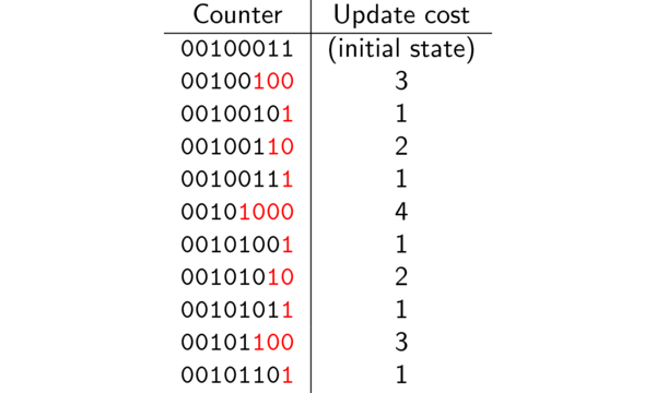
8-bit counter increments
If you look at some examples and actually do the binary counting (like we did in class), you'll discover that:
D[0](the least significant bit) changes at every incrementD[1]changes every other incrementD[2]changes every fourth incrementD[3]changes every eighth increment- In general,
D[i]changes every \(2^i\)th increment
This means that, in any sequence of m increments, digit i will be updated at most \(\lceil m/2^i\rceil\) times. The total cost of all the increments is just the total cost of all the times each digit gets changed. So to count this total cost, we can add up the worst-case number of updates of each digit, over all k digits:
\[ \sum_{i=0}^{k-1} \left\lceil\frac{m}{2^i}\right\rceil \le \sum_{i=0}^{k-1} \left( 1 + \frac{m}{2^i}\right)\le \sum_{i=0}^{k-1} 1 + m\sum_{i=0}^{k-1}\frac{1}{2^i} \]
Now you didn't forget how to solve summations did you? The left one is easy — it just sums up to the number of things in the summation, which is k. For the right-hand summation, notice that this is a geometric series, and no matter how large k is, it will never be greater than two. So the whole thing sums up to \(k + 2m\).
Remember that this is the total cost for all m increments. The amortized cost is defined as the total cost, divided by m, which for this algorithm comes out to \(2 + k/m\). To get rid of the pesky \(k/m\) part, we can make any one of three very reasonable assumptions: either k is a constant, or \(m\ge k\), or the counter starts at 0. If any of these conditions is true, then the amortized cost of incrementing the counter is just \(\Theta(1)\) — constant time!
Now take a step back and consider what we've learned. If we consider just the worst-case cost of the increment operation, it's \(\Theta(k)\), the size of the counter. But if we do a bunch of increments in a row, the overall situation is exactly the same as if each increment only cost constant time. Awesome!
3 Self-Organizing Search
Now let's look at a different problem, called "self-organizing search", or sometimes the "list update problem". The basic idea is to store some elements in an array, and then we will have a sequence of "lookup" operations to access these array elements. In reality, each element will be a key-value pair, and the lookup will be based on the keys and return the corresponding value. For our examples, we'll just draw out the keys, for simplicity.
Since the array elements won't be sorted in order, each lookup will be by a linear search. Remember that? It's the first algorithm we looked at on day one of this class! For example, if the array looks like
\[[52,32,96,73,50,27,16,31]\]
then looking up key 73 requires looking through the first four list elements. In general, the cost of looking up any key is proportional to the position of that key in the array.
Nothing new here so far — this just sounds like a basic (bad) implementation of the Map ADT. What's special is the "self-organizing" part. That means that, after each lookup, we are allowed to re-order the list any way that we like. Of course the goal is to perform these re-orderings in such a way that future look-ups will be less costly.
Essentially, we'll use the information of which elements have been searched for so far to predict which elements are most likely to be searched for next. The very best way to do this would be to keep counts of every element and order them based on those counts — but this isn't allowed (it would take too much space). All we are allowed to do is reorder the elements, so that more frequently searched-for ones are closer to the front of the list.
Here's a concrete example of why we might want to do something like this: Google. There are millions of possible searches, but they're definitely not all equally likely. We want to keep the more likely searches near the front of the list. (Disclaimer: Google's actual search algorithms are way, way more complicated than what we're discussing here. It's just an illustration.)
3.1 Move to Front
The first re-ordering strategy we might consider is called Move to Front (MTF). And it works just the way it says: every time an element is looked up, it gets moved to the front of the list. For example, if the element with key 73 is looked up in the array above, it will be immediately re-ordered so that 73 is in front, and all the intervening elements are pushed back:
\[[73,52,32,96,50,27,16,31]\]
Then if 50 were searched for, we do the same thing again, ending up with:
\[[50,73,52,32,96,27,16,31]\]
But now if 73 is searched for again, it's really fast to find it (and to move it to the front). MTF is all about making drastic changes, but if we search for the same element many times in quick succession, all the searches except possibly the first one will be really quick.
3.2 Transpose
Transpose is a less drastic update method. Whenever an element is looked up, we swap it with the one immediately preceding it in the list (unless it's already at the front. Here's how it works for the same example as above. We start with
\[[52,32,96,73,50,27,16,31]\]
Then searching for 73 updates this to
\[[52,32,73,96,50,27,16,31]\]
Looking up 50 next gives
\[[52,32,73,50,96,27,16,31]\]
And another lookup on 73 changes this to
\[[52,73,32,50,96,27,16,31]\]
So you see, transpose is all about making small incremental changes that (hopefully) slowly push the more frequently searched-for elements towards the front of the list. The potential advantage here is that, if an element is only searched for once, we don't immediately bring it all the way to the front, only to have it get in the way of all the subsequent searches.
4 Analysis of List Update Strategies
So which one of these list update methods is better? Is there any way to make this judgement? In order to do the analysis, we have to define some more parameters:
- n is the number of elements in the list
- m is the number of searches. Generally, we can assume m is much larger than n.
- The frequency of each element is the number of times it is looked up. We'll write \(k_1, k_2, \ldots, k_n\) for the frequencies of each of the n elements. Notice that the sum of the \(k_i\)'s must equal m.
4.1 Optimal Static Ordering
The way our analysis is going to work is by comparing each of the two update methods above (MTF and Transpose) with the optimal static ordering. This is the best possible way to order the array, if we knew in advance which elements would be searched for.
And what is this optimal static ordering? Easy — just order the elements by their frequencies, which the most frequently-searched element in the front of the list, followed by the next most frequently looked-up one, and so on, until the least frequently looked-up element which is at the end of the list.
Call this ordering OPT. We will compare the cost of a sequence of searches using MTF and Transpose, to that same sequence of searches if the ordering is fixed at OPT. The algorithm whose performance is closest to OPT wins!
4.2 Average Analysis
Transpose looks really good here because, after enough searches, there's a very good chance that the array that gets reordered by the Transpose operation actually ends up in exactly the same order as OPT, and then stays in (roughly) that same order.
Formally, this argument is doing something like an average-case analysis. Considering all possible sequences of searches with a given set of frequencies \(k_1\) through \(k_n\), if we assume that each possible search sequence is equally likely, then the average cost using Transpose will be the same as the cost of OPT, after accounting for the initial look-ups necessary to "settle" the array into its proper order.
This fact was first noticed by none other than Ron Rivest, of RSA fame, who wrote an important paper analyzing Transpose and concluded that it had better performance than MTF for the reasons described above, and in fact conjectured that Transpose was the best possible list update algorithm.
But something funny happened: this didn't agree with experience. People actually working in various database-type applications observed that MTF seemed to work better in practice compared to Transpose. So the best algorithm in theory, wasn't the best one in practice.
4.3 Theory versus Practice
When this happens — theory disagrees with practice — what it really tells us is not that the theoretical result is "wrong", but rather that the assumptions we made were wrong. And what assumption got made in the analysis above? The same incorrect assumption that always gets made for average-case analysis: that every possible ordering (of look-ups) is equally likely! In reality, this is absolutely not the case for most applications: searches for the same element tend to be somewhat clustered in time, rather than spread out evenly.
For example, there were probably a lot of Google searches for the word "tax" in the first two weeks of April, not so much in the first two weeks of August. If we just considered the total quantity of searches for "tax" and said these are spread somewhat evenly throughout the sequence of searches, this is a really bad assumption!
And this is also the main advantage of MTF: it takes good advantage of temporal locality in the look-ups. So yes, MTF might make some bad choices by moving infrequently searched-for elements to the front, but by definition this will happen infrequently! The advantages we get from MTF seem to outweigh the drawbacks.
4.4 Competitive Analysis
So do we give up the fight and just say, "MTF seems to be better in practice, but we can't really say exactly why"? Never! The shortcomings of our theoretical analysis were bad assumptions, so by making more reasonable assumptions (or just fewer assumptions altogether), maybe we can get more meaningful results.
This is where competitive analysis comes in, and where we tie this discussion back to the ideas of amortized analysis. Competitive analysis again compares each update method to the optimal static ordering OPT, but instead of looking at the average over all search sequences, we just look at the worst-case sequence of searches, and see how the performance compares to that of OPT. Remember the basic principle of analysis: if the worst-case is pretty good, then every case is pretty good!
One nice property is that the way we do competitive analysis is essentially the same as that for amortized analysis, because in both cases we're looking at the total worst-case cost for a sequence of m operations on some continuously-updating data structure.
The first thing to figure out is how Transpose does in the light of competitive analysis. And the answer is: really, really bad. The very worst case for Transpose is that we keep alternating searches between just two items in the list, like looking up 31, then 16, then 31, then 16, and so on for all m searches. Well if these two elements happen to start out at the end of the list, like:
\[[52,32,96,73,50,27,16,31]\]
then every Transpose update just swaps these two elements! So each of these m searches will cost \(\Theta(n)\), for a total cost of \(\Theta(nm)\) for all the searches. Now for competitive analysis, we want to compare this to OPT, so how would this list be ordered if the items were sorted by lookup frequencies? 16 and 31 would be the first two elements of the list, so each search would cost \(\Theta(1)\), total of \(\Theta(m)\).
In other words, in the worst-case, Transpose is n times worse than OPT. So even though Transpose looks good for a random search ordering, it can easily be "tricked" into giving the worst possible behavior — really, really bad!
By now you should expect that MTF will be better. Here's why. Consider any sequence of requests with frequencies \(k_1, k_2,\ldots, k_n\), as before. The cost of each lookup for some element i is equal to the number of elements that precede i at the time when it is searched for. Sum up the number of elements preceding each i, at every search, and we have the total cost for all m searches.
The cool thing about MTF is that we can actually do this analysis by just considering two elements at a time, say element i and element j. We will add up the number of times j precedes i when i is searched for, and vice-versa. By adding up all these for every pair of elements, we get the total cost of all the searches, just like before!
So now consider i and j, and assume \(k_i \ge k_j\), that is, assume i is the more frequently looked-up element of the pair. What is the number of times j precedes i when i is searched for, in the worst case? You might be tempted to say "every time", but that's not possible because i gets moved to the front after each of its searches, and this means it will be moved in front of j. Since i is searched for more frequently than j is, i must be in front of j at least some of the times it gets searched for.
So the real limit to the number of times j could precede i in a search for i is the number of times j could get moved in front of i, which is \(k_j\), plus one for the initial search for i.
And what about the number of times i could precede j in a search for j? This time the answer really is "every time", which means \(k_j\) again. So the total cost for the pair \((i,j)\) is at most \(2k_j+1\).
Remember that for competitive analysis we're supposed to compare this to the cost of OPT, the optimal static ordering where elements are ordered by decreasing frequency. We could add up the total cost of MTF and OPT and compare them, but it will easier to instead compare the cost for each pair, and sum those up.
So for the same pair of elements \((i,j)\), how often in OPT does j precede i in a search for j, or vice-versa? Well, since i is more frequent than j, it will come before j in the optimal static ordering, and therefore j never precedes i. But i does precede j in every single search for j, which means a total cost of \(k_j\) for this pair.
Therefore we have \(2k_j+1\) as the total cost per pair for MTF, and \(k_j\) as the total cost per pair for OPT. Assuming (reasonably) that every element is searched for at least once, \(k_j\ge 1\), and therefore \(2k_j+1\le 3k_j\). This means that the cost for MTF is at most 3 times more than the cost for OPT. Summing this over all the pairs, we will get the total worst-case cost for both MTF and OPT, but the ratio will always stay the same, 3. In other words, in the worst case, for any sequence of searches, MTF is at most 3 times as bad as OPT.
In fact, a more sophisticated (difficult) analysis can be used to show that MTF only performs at most 2 times as much work as any other list-update strategy, even one that's allowed to know all the look-up requests in advance and take exponential time to re-order the list. So we say that MTF is "2-competitive", and give it its rightful credit as the most efficient method for list update, both in theory and in practice!
5 Finale
Even if some of the details of the analysis above are a bit hazy, it's important to recognize what happened: we had one analysis that disagreed with practice, then by reexamining the underlying assumptions in that analysis, we came up with a different one that confirms our experiences. And there's much more to it than just confirming what we already know — the idea of competitive analysis has now been used on a wide variety of problems to come up with many efficient algorithms. So it all comes down to algorithms, analysis, and implementation, and they're all constantly affecting each other and bringing us to newer and greater heights of algorithmic nirvana!
Congratulations on reaching the end of the notes. I hope you've enjoyed the journey as much as I have. As a special gift, if you include the word "Sousaphone" in your Daily Quiz submission for today's class, I'll turn your lowest DQ grade into a 3. (You still have to answer the DQ though!)