1 Overview

From the earliest days of computing, people have wanted to store and transmit data using less space or bandwidth. Compression algorithms are ways of representing the same information as a large data file using less space.

You are probably familiar with many file formats that use compression, such as .zip, .gz, .png, .jpg, .mp3, and .mp4. Compression is also used to transmit much of the HTML, Javascript, and CSS source code for web sites you visit.

In this unit, we are going to learn about how some of these compression techniques work. We typically think of “data structures” as things that reside in computer memory (RAM), and not long-term storage like files. But the ways of thinking about compression draws on many of the same concepts like data organization and big-O runtime. Furthermore, many of the compression schemes use some of the interesting data structures we have learned about, such as trees, tables, and heaps. So we hope this unit will be a nice way to wrap up the semester.

1.1 Lossy and Lossless

At a very high level, all compression schemes consist of two algorithms: compression and decompression, which work as shown in this diagram:

When we say “file”, think of these as just streams of bytes — they could be actual files on disk, or data that’s about to be sent over a network connection, for example.

When the decompressed file is always exactly identical to the original file, the compression scheme is called “lossless”. Otherwise, if the decompressed file is similar to, but not exactly the same as, the compressed one, the scheme is called “lossy”.

Lossy compression is commonly used for data that comes from physical sensors, like raw images, audio, or video. In fact, some formats like JPEG allow you to specify the compression level explicitly when saving an image. For example, below you can see an image of a turtle in Dr. Roche’s back yard, with three different levels of JPEG compression (click here for a bigger version):

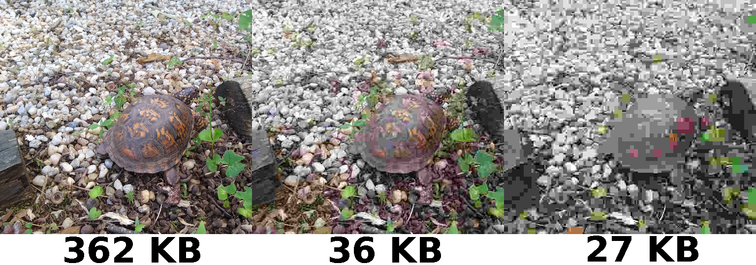
Notice that we can get quite a lot of compression before the image starts to really look “bad”, which is because real-life images are pretty predictable, with lots of repeated colors and small patterns. But at some point, the compression is too much and the image is almost unrecognizable.

Lossy compression makes a lot of sense for images, sounds, and movies, but the techniques are as much about human perception as they are about computer science techniques. Furthermore, these techniques are very specific to the type of media you are compressing: you wouldn’t want to use an audio compression technique for an image, for example.

For these reasons, lossy compression is almost never applied to text. Consider, for example, this passage from Catch-22 by Joseph Heller which has been compressed down to 85% of its original size by dropping some random letters:

All teoffice tents inthewar werorc to cenor letteswritn byll theenlis-men ptients, who erekptin esidence in wardsofthei own.It was amontoous jo, andYosarian was disapointed to lern that the lives of nlisted men ere only slightl moeineesting than the lies o ffcers. After the first day hehad no urioit at al. To break the monotoy he invnted games. Death to all modifers, he declared on a and out of ery lett ht ase thrug hs hands nt evey aderb an evry adjectie. The nextday he made waon aricles. He reachd amuchhigher lane f creativity te foloing day when he backdut everything in th letersbuta, a andthe.

You can probably make out somewhat what the original text is saying, but it’s difficult. Another approach to “lossy” text compression would be using AI, as in this machine-generated “summary” of the same passage:

Yossarian was ordered to censor letters written by all the enlisted-men patients, who were kept in residence in their own ward. After the first day he had no curiosity at all. To break the monotony he invented games. He reached a much higher plane of creativity the following day when he blacked out everything in the letters but the letters.

Here it’s actually easier to make out the gist of what the original passage is saying, but I don’t think you would want to read a novel written this way. (Notice some wonderful phrases which are just lost entirely: “the lives of enlisted men were only slightly more interesting than the lives of officers”, “Death to all modifiers”, “war on articles”.)

And even if you have no taste for word artistry and think lossy compression of books would be okay, imagine the havoc this would wreak on other plain-text files such as source code!

For these reasons, compression of plain-text files is almost always lossless, and those are the kind of algorithms we will focus on in this unit. Another advantage of studying lossless compression algorithms is that they can be applied to any kind of file, not just a images or just audio. The lossless compression schemes we will learn are similar or identical to those used on web sites, for ZIP, GZ, and BZ2 archives, and for GIF and PNG images.

1.2 Analyzing compression schemes

There are four main factors we use to judge a lossless compression algorithm:

1. Correctness: Do the compression and decompression algorithms work to perfectly recover any possible input file?
2. Compression ratio: How much smaller is a “typical” compressed file compared to the original?
3. Decompression speed: Worst-case big-O runtime of the decompression algorithm.
4. Compression speed: What is the worst-case big-O runtime of the compression algorithm, in terms of the size of the original file?

Usually we care about them in this order. Note that decompression is more critical than compression for speed (usually), as the same file can be compressed once but later decompressed many many times.

We have discussed correctness and worst-case big-O running times repeatedly throughout the semester, but the way we will think about the compression ratio is a bit different. Here is a definition:

\[\frac{\text{size of original file}}{\text{size of compressed file}}\]

For example, a compression ratio of 1.5 on a 30MB file would bring the size of the compressed file down to 20MB.

We should care about the worst-case and best-case here, but usually that doesn’t tell the full picture. In any lossless compression scheme, the worst-case compression ratio will actually be less than 1 (a slight expansion) — can you see why that is the case? So worst-case is not very useful here. Similarly, I can easily construct a “bad” compression algorithm that has a great best-case:

Bad compression algorithm with great best-case compression ratio

If the file contains “ABCDEFGHIJ” in order, 1 million times, represent it as “1”. Otherwise, represent the file by “0” followed by the actual file contents.

That algorithm will have a very poor compression ratio of \(\frac{n}{n+1}\) for almost every length-\(n\) file, except for one very specific file where the compression ratio is 10,000,000:1. So the best-case is wonderful, but it’s obviously pretty useless.

For this reason, we usually focus on “typical” compression ratios for real-world files. In this unit, we’ll focus mainly on some books and song lyrics when considering the compression ratios of different algorithms. It’s a little less mathematical and more empirical than the big-O analysis we have been looking at most of the semester, but sometimes this is the most helpful way to compare computational processes.

2 Run-Length Encoding (RLE)

The first and simplest compression algorithm is actually not very useful on its own for most kinds of data files, but it is useful in combination with some others, and is a simple algorithm to help get us started.

For RLE, we encode any sequence of bytes as a list of pairs \((x,k)\), where \(x\) is a single byte, and \(k\) is the number of times that byte is repeated. So runs of repeated, identical bytes are replaced with a single pair. For simplicity, we’ll limit the run length \(k\) to also be a single byte, so an integer from 1 up to 256.

For example, here is a random length-16 DNA sequence:

ggggaataaaaaggtc

Its RLE encoding consists of 7 pairs:

(g,4)
(a,2)
(t,1)
(a,5)
(g,2)
(t,1)
(c,1)

Treating everything as bytes, in this case the RLE encoding transformed a 16-byte input to a 14-byte compressed output, for a modest compression ratio of \(\frac{16}{14}\), or about 1.14.

That’s all there is to it! As we said, RLE is pretty simple. Let’s think about how to analyze it:

• Correctness: Any possible byte sequence can be encoded and decoded.

• Compression ratio: The worst case would be no runs at all, so every \(k\) value would be 1 and the compressed size would be \(2n\), for a terrible compression ratio of 0.5.

  The best case is that all characters are the same, for a maximum compression ratio of 128 (using single-byte values for the run lengths).

  For “typical” English text files, there are not very many repeated letters, and the compression ratio of just using RLE is close to the worst case. However, it can be very effective on certain kinds of images and in combination with other techniques we’ll discuss later.

• Decoding speed: The algorithm just requires a single pass through the pairs, \(O(n)\).

• Encoding speed: Also \(O(n)\) with a single pass through the input.

3 Lempel-Ziv-Welch (LZW)

Abraham Lempel and Jacob Ziv are two Israeli computer scientists who developed a number of compression algorithms in the 1970s that form the basis of much of what we use today. The most important variant is called LZ77 and is used in the zip file format (among others)

The key insight of Lempel-Ziv based compression algorithms is that sequences of bytes in the uncompressed file are likely to happen again later in the file. This sort of encompasses the idea of RLE but makes it much more general: the repetitions can be multiple characters long, and they don’t have to be right next to each other. It turns out that this kind of repetitive structure appears in many different kinds of documents, which is why Lempel-Ziv is the basis for the most general lossless compression algorithms.

We will look at a slightly simpler-to-implement variant called LZW which was developed in 1980 along with the American computer scientist Terry Welch. LZW compression is still used in the GIF image format, and shares a number of key ideas with the older LZ77 algorithm on which it’s based.

3.1 Table-based encoding

LZW is a table-based encoding, meaning that both the encoder and decoder use a lookup table to translate input symbols to output symbols.

In LZW, each encoded symbol is a 12-byte number, from 0 up to 4095. Each 12-byte symbols can represent one or more decoded bytes.

For example, with this encoding table:

Encoded symbol	Decoded string
46	.
84	T
104	h
110	n
260	ra
263	n␣
272	al
286	␣p
293	e␣r
297	Spa
300	fal
303	mai
305	ly␣
317	in␣f
319	ls␣
323	on␣
325	the
332	ain␣i
340	he␣pl
341	lai

Then the 44-character sentence

The␣rain␣in␣Spain␣falls␣mainly␣on␣the␣plain.

Can be encoded with the following sequence of just 18 encoded symbols:

84 104 293 332 263 297 317 272 319 303 110 305 323 325 286 341 110 46

What is the compression ratio in this example? Naively, you might think it is \(\frac{44}{18}\), about 2.44. However, this does not account for the fact that each encoded symbol is 12 bits, meaning that every 2 encoded symbols take up 3 bytes in the file. So those 18 symbols actually take up 27 bytes of memory, bringing the actual compression ratio in this example to \(\frac{44}{27}\), which is about 1.63.

3.2 Generating the table

OK, so the question is, how do we get the table itself? Why not just put the whole file we are encoding as a single entry in the table and call it a day?

The reason is that we do not want to store the table in the compressed file, only the list of encoded symbols. This means that the compression and decompression algorithms must both use the same table, without explicitly communicating it.

One way to do this might be to make a big pre-computed table, say, of common English words and phrases. But there are two problems with this approach. First, that table would be far too big, and the resulting encoded symbols would be longer than 12 bits each. Second, it would be too specific: we want to create a compression algorithm that works well for any input, not just for English language plain-text files.

Instead, the insight of LZW is that the encoder and decoder both just build the table as they go. Remember, the key insight of all Lempel-Ziv compression is that sequences of bytes are likely to recur again later in the file. So with LZW, we save sequences as we go, so they can be referred to later.

Every time a sequence recurs later in the file, we add one more character and add that new sequence to the table, so that when it recurs again, we might be able to use the even longer encoding.

3.3 Encoding

Specifically, the encoder works like this:

1. Initialize the table with all single-byte values, encoded as 0–255, and with a total of \(2^{12}=4096\) rows available.
2. Take the longest sequence from the input that is encoded in the table, \(S\), and add the numerical encoding of \(S\) to the output.
3. Peek ahead at the next byte \(b\) in the input, and insert the concatenated string of \(S+b\) at the next available row in the table (unless the table is already full).
4. Repeat steps 2 and 3 until the input reaches end-of-file.

What happens in “typical” text files is that, initially, all of the output encodings are single ASCII characters, and the table entries added are all pairs of letters. But then a pair of letters repeats, gets encoded, and we add a three-letter combination to the table. After a while, the table contains all of the multi-byte combinations that are most common in the file, and these can be efficiently encoded from that point forward.

As an example, consider the encoding of the lyrics to the Beatles’ All you need is love, which begins pretty repetitively:

Love, love, love
Love, love, love
Love, love, love
...

Let’s see how to encode this using LZW.

• Initially, the table has all single-byte values (ASCII table) from 0 up to 255.
• The first encoded string is L which has ASCII code 76.
• Right away, we tack on the next letter and add Lo to the table with code 256.
• Next, starting with the o (which was added to the table, but not yet encoded), the longest string in the table starting from this spot is just o, ASCII code 111. We add ov to the table with code 257.
• Similarly for the next five characters, each are encoded with their single-byte ASCII code, and the two-byte sequences ve, e,, ,␣, ␣l, and lo are added to the table with codes 258–262.
• The next unencoded input byte is the second o, but now there is a longer substring that exists in the table: ov with code 257! So we output code 257 and add the three-character substring ove to the table with code 263.

Here is a table summarizing these initial steps of the LZW encoding for the song lyrics:

Input substring consumed	Output code	New table entry	New code
L	76	Lo	256
o	111	ov	257
v	118	ve	258
e	101	e,	259
,	44	,␣	260
␣	32	␣l	261
l	108	lo	262
ov	257	ove	263
e,	259	e,␣	264
␣l	261	␣lo	265
ove	263	ove\n	266
\n	32	\nL	267
Lo	256	Lov	268
ve	258	ve,	269
,␣	260	,␣l	270
lo	262	lov	271
ve,	269	ve,␣	272
␣lo	265	␣lov	273
ve	258	ve\n	274
\nL	267	\nLo	275
ove	263	ove,	276
,␣l	270	,␣lo	277
ove,	276	ove,␣	278
␣lov	273	␣love	279
e	101	e\n	280

Notice how the encoding gets better as it goes along and the table is filled in. Each line `Love, love, love” has 17 characters in the input. The first line takes 12 symbols to encode it, but the second line only 8 symbols, and the third line only 6.

You can peruse the entire encoding of the lyrics here. The final result is that 1812 bytes of input get compressed to 554 12-bit symbols, for a total compression ratio of

\[\frac{1812}{554\cdot\tfrac{3}{2}} \approx 2.18\]

3.4 Decoding

LZW decoding works almost exactly the same as encoding. We start out with a table of single-byte ASCII values, then enter a loop where each iteration does three things:

1. Reads then next encoded symbol from the compressed file
2. Looks up that symbol in the table and outputs the decoded bytes to the output
3. Adds a new table entry with the previously decoded byte sequence plus one more byte.

Except there’s a problem: for this third step we don’t know the next byte yet until the next symbol is decoded! So the decoder’s table is always “one symbol behind” where the encoder would be; we normally have to wait until the next symbol is decoded to add something new to the table.

This is all good except in one special case: when the encoded symbol is not yet in the decoder’s table. That happens specifically because of the decoder being “one behind”; the encoder outputs the last table entry, but the decoder doesn’t have this table entry yet. What to do?

Remember that the decoder knows almost the entire output sequene of this next table entry, but it’s just waiting for the last byte to be added on. But now we know the next byte will be the first byte of that output sequence, so we can add it to the table early, and it’s all good.

In other words, when the next encoded symbol is not yet in the table, we add the previous decoded sequence plus appended with its initial byte to the table, and output that on step 2.

I realize the description above is probably a little confusing, so let’s look at an example. Here is an LZW encoding:

78 79 32 256 258 257 259 262 257 89 69 83

The decoder starts with a table of the 256 single-byte values, numbered 0 up to 255 (same as the encoder started with).

The first encoded symbol 78 is the ASCII code for N, so we add that to the output and remember it. (We are not yet ready to add any new table entry, since we don’t know the next output character yet.)

The next encoded symbol 79 is the ASCII code for O. So we add that to the output and append the first character to the previous output and add that to the table, at index 256. So now we have:

Table:
256 NO

Output:
NO

The next encoded symbol is 32, an ASCII space character ␣. We add this to the output and append its first character to the previous output to get the next table entry.

Table:
256 NO
257 O␣

Output:
NO␣

The next symbol is 256, which is not a single character but rather the first one from the table we are building as we go. LZW is actually doing a little compression here! The table tells us 256 is the string NO, so we add that to the output, and append its first character N to the previous output ␣ to get the next table entry.

Table:
256 NO
257 O␣
258 ␣N

Output:
NO␣NO

The next encoded symbol is 258. This is in our table, so we add its decoding ␣N to the output, and append its first symbol ␣ to the previous output NO to get the next table entry.

Table:
256 NO
257 O␣
258 ␣N
259 NO␣

Output:
NO␣NO␣N

The next two encoded symbols, 257 and 259, work similarly: we add O␣ and then NO␣ to the output, and two more entries to the table.

Table:
256 NO
257 O␣
258 ␣N
259 NO␣
260 ␣NO
261 O␣N

Output:
NO␣NO␣NO␣NO␣

The next encoded symbol is 262. UH OH, WE’VE HIT THE SPECIAL CASE! 262 is the next table entry which hasn’t been added yet. We know that that table entry starts with the previous output NO␣ but the next character needs to be added. In this special case, we know that the next character will be the first byte of this output, which in this example is N. So we can prematurely add this table entry by appending its first character to the end, then output that value:

Table:
256 NO
257 O␣
258 ␣N
259 NO␣
260 ␣NO
261 O␣N
262 NO␣N

Output:
NO␣NO␣NO␣NO␣NO␣N

The next encoded symbol is 257. We’re back to the normal case: this is already in the table, so we ouptut its decoding O␣ and add its first letter to the previously-output decoding to get the next table entry:

Table:
256 NO
257 O␣
258 ␣N
259 NO␣
260 ␣NO
261 O␣N
262 NO␣N
263 NO␣NO

Output:
NO␣NO␣NO␣NO␣NO␣NO␣

The final three encoded symbols 89, 69, and 83 are single-character ASCII decodings, which also cause three more table entries. (We know these table entries won’t be used, but the decoder still generates them.)

Table:
256 NO
257 O␣
258 ␣N
259 NO␣
260 ␣NO
261 O␣N
262 NO␣N
263 NO␣NO
264 O␣Y
265 YE
266 ES

Output:
NO␣NO␣NO␣NO␣NO␣NO␣YES

This completes the decoding, so we can throw away the table and just return the output itself. All in all, the 12 input symbols (comprising \(12*\frac{3}{2}=18\) bytes) decoded to 21 bytes of decompressed output. The compression ratio was therefore \(\frac{21}{18}\approx 1.17\).

4 Huffman Coding

Huffman coding is another compression technique that is used to turn a stream of bytes (or any stream of numbers) into a stream of bits. Like LZW, Huffman coding is table-based, but it’s kind of the opposite: instead of fixed-length encoding symbols which correspond to varying-length decoded substrings, Huffman associates each individual symbol (e.g., each byte) from the input with a variable-length string of bits.

For example, consider the following 12-byte input:

BANANACABANA

How would we encode this to bits?

Using ASCII, as the original input likely is given, each character is stored using 8 bits, for a total of \(12\times 8 = 96\) bits.

Right away you should be able to think of a better solution. Notice that there are only four letters that actually appear in the string. So we could arbitrarily assign a different two-bit pattern to each of these letters, and then encode using that:

Original Character	Encoding
A	00
B	01
C	10
N	11

Then the original 12-byte (96-bit) string can be written using only 2 bits per character, or 24 bits total, as:

 B A N A N A C A B A N A
010011001100100001001100

Notice that we’ve assigned each input byte to the same length bit string in this example. But that isn’t necessarily the best option! In this case, the letter A appears most frequently in the input, and C appears last frequently. So if we could assign fewer bits to each A and more bits to each C, that would be a good trade-off. Here is an encoding table that does that:

Original Character	Encoding
A	0
B	100
C	101
N	11

This slight improvement allows us to use only 21 bits to encode the entire string:

  BA NA NA  CA  BA NA
100011011010101000110

As it turns out, this variable-length encoding is exactly what the Huffman algorithm will give us.

In terms of decoding, notice that we just get the table above and a continious string of bits — it’s not immediately clear how the decoder will know where each encoding ends and the next one begins. But in fact the encoding table above has a special property that means there is only one possible decoding: it is prefix-free. What that means is that each of the encoded character sequences (0, 100, 101, 11) is not a prefix of any other sequence. Huffman encoding actually generates a prefix-free coding of the original bytes that results in the minimal number of encoded bits.

Let’s see how it works!

4.1 Huffman Trees

Because the Huffman encoding table is prefix-free, it can be represented by a binary tree with the following properties:

• Every input character (byte) is a leaf of the tree
• Every non-leaf node has exactly 2 children
• The left child corresponds to a 0 bit, and the right child corresponds to a 1 bit.
• The path of 0’s and 1’s from the root to a leaf is exactly the bit-encoding of the character at that leaf.

This data structure is called the Huffman tree for the given encoding. (It is technically a trie built on the alphabet of 0 and 1.) Here is the Huffman tree for the previous example:

The structure of the tree actually guarantees the prefix-free property of the code, since only leaf nodes have labels.

4.2 Generating the tree

We have seen that Huffman trees show us how to encode and decode, and that, generally speaking, we want more-frequently-appearing characters to have lower depth (shorter encodings), and less-frequent characters to have higher depth (longer encodings).

David Huffman figured out the optimal way to create this tree in 1952 (the same year Grace Hopper published a paper describing the first programming language and compiler). Huffman’s method is so simple and elegant that it is still in use today.

Here is the algorithm:

1. Make one pass over the input to find the frequency of every character (byte)
2. Create a separate subtree for each character, each of which initially consists of a single leaf node, tagged with that character’s frequency.
3. Remove the two subtrees with the lowest frequencies and combine them as the two children of a new internal node. Associate this new subtree with the sum of the frequencies of its two children.
4. Repeat step 3 until there is only one subtree left. That is the Huffman tree.

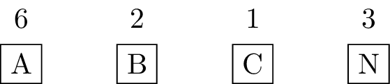
Let’s work this through with the BANANACABANA example. First we compute frequencies and create 4 leaf nodes for the 4 characters that appear in this string:

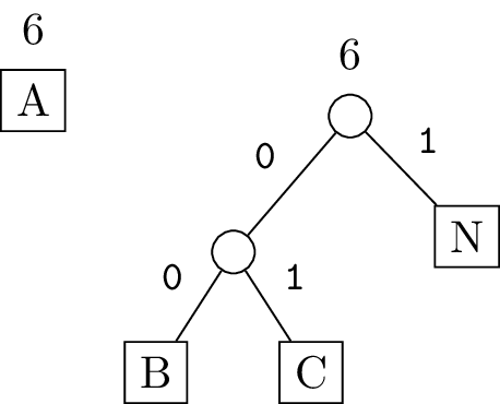
B and C have the lowest frequencies, so we combine them into a new subtree with frequency \(2+1=3\):

Now the lowest two frequency subtrees have weight 3, so we combine them next:

There are now just two subtrees left, so we combine them to get the entire Huffman tree:

4.3 Encoding algorithm details

We just saw one example, so let’s make a few things clear:

• In this example, we always combined subtrees with exactly equal weights, but it won’t always work out that perfectly. Just remember that you always combine the two subtrees remaining that have the smallest weights.

• The left/right ordering doesn’t really matter in terms of encoding length. For example, we could also use this tree to encode BANANACABANA and get the same length (with a different bit pattern):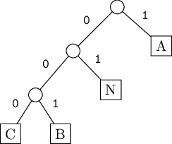

  

• The subtrees to combine won’t necessarily be “next to” each other. Remember, you always want to combine the two subtrees with the smallest weights at each step.

• There can be duplicate frequencies/weights among the subtrees at any point, so the choice of two subtrees with smallest frequencies/weights might not be unique. In that case, it doesn’t matter which two smallest-frequency subtrees get combined — either way will result in the same final encoding length.

What data structure do you think we should use to keep track of these subtrees? We need to be able to insert things, and remove the smallest things… sounds like a priority queue! Usually a heap is used, since that’s the best general data structure when we need to do lots of insertions and removals from a priority queue.

Overall, the entire encoding algorithm looks like this:

1. Make one pass over the input and compute the frequencies of each symbol (byte or character)
2. Construct the Huffman tree using those frequencies
3. Make an in-order traversal of the tree to generate an encoding table like shown above, associating each byte or character to its multi-bit encoding.
4. Make one more pass through the input, encoding each character to the output.

Suppose the input has length \(n\) and contains \(m\) unique bytes or characters. Steps 1 and 4 both cost \(O(n)\), step 2 costs \(O(m\log m)\) if using a heap, and step 3 is \(O(m)\). So the total cost is \(O(n + m\log m)\).

(If we are really dealing with bytes, then \(m\le256\) is a constant, so we could just say \(O(n)\).)

4.4 Encoding the tree itself

Well actually, one step is left out. Besides encoding the bit pattern for the actual input encoding, we also need to add the Huffman tree itself to the encoded file. Unlike LZW, it is not possible for the decoder to just figure this out as they go; the Huffman tree needs to be sent explicitly.

There are multiple ways to do this, but for large files it won’t make a big difference in the overall output size, since the tree only has \(2m-1\) nodes. Here is one way to encode the Huffman tree:

• Perform a pre-order traversal of the tree
• Each time an internal node is visited, output a 0 bit.
• Each time a leaf node is visited, output a 1 bit, followed by the single-byte label on that leaf node.

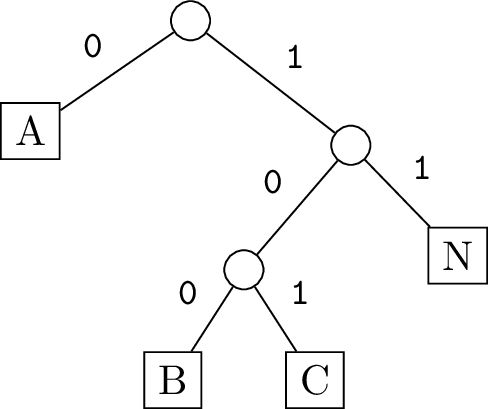
Under this scheme, the following tree:

would be encoded as

01A001B1C1N

Of course, in reality each of A, B, C, N would actually be an 8-bit pattern for that corresponding byte (ASCII) value.

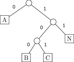
By contrast, this tree which is equivalent length-wise but uses a different structure:

would be encoded as

0001C1B1N1A

Either way, encoding the tree in this way takes \(O(m)\) bits.

4.5 Decoding

The Huffman decoding process is pretty simple. You just have to decode the tree, then follow the 0/1 branches of the tree as you read the rest of the bits to decode each byte of the original file.

Let’s do an example! Consider this Huffman encoding (which starts with the tree encoding, then the actual bits of each encoded character):

001B1D01A01I1S1001011101111000100010

First we have to decode the tree, which is this part:

001B1D01A01I1S

Remember, this is a pre-order traversal, where the 0’s are internal nodes (all of which have exactly two children) and the 1’s are leaf nodes (followed by their label). So it works out to this Huffman tree:

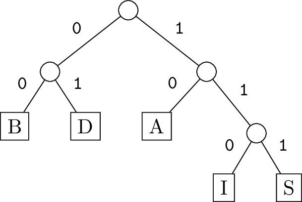
What remains is the encoding of the actual bytes of the original file:

1001011101111000100010

To decode this, we use our tree, starting at the root and following edges according to each bit. When we reach a leaf, output that character and go back up to the root.

The first few bits are 10 which goes to A, then 01 which goes to D, another 01 for another D, and then 110 for I. Here is how the whole process breaks down:

10 01 01 110 111 10 00 10 00 10
 A  D  D   I   S  A  B  A  B  A

And therefore the original file was ADDISABABA.

4.6 Compression ratio

Huffman coding is effective at the level of individual characters, and is therefore useful for things like English text where some letters (“e” for example) are much more likely to appear than others (“q” for example, or symbols such as “~”).

By itself, Huffman usually achieves a compression ratio around 1.7 on English text compared to the default ASCII encoding. That’s pretty good, but a little worse than LZW, because LZW is able to recognize not just individual characters that are frequent, but entire sequences (e.g. common English words).

The reason Huffman is still relevant is that it is almost always used in composition with another encoding algorithm. The popular ZIP file format, for example, mostly uses the LZ77 compression algorithm, followed by Huffman encoding. In fact, Huffman is usually the last step in a compression algorithm.

Here is a comparison of compressing the lyrics to every Beatles song using LZW by itself, Huffman by itself, and then LZW followed by Huffman. (The lyrics are originally stored in 277KB.)

Algorithm	Compressed Size	Compression Ratio
LZW	141K	1.962
Huffman	160K	1.728
LZW+Huffman	129K	2.140

So we see that LZW+Huffman achieves better compression than either one individually. Thinking about how LZW works, at some point in the encoding, there will be an encoded symbol for a common word like “the”. And this encoded symbol (a 12-bit number) will appear many times in the LZW output. Then Huffman comes in to save the day — whatever the LZW table index for “the” is, will probably have higher frequency than other values, and therefore end up with a shorter bit-length encoding via Huffman.

5 Burrows-Wheeler

The last compression algorithm we will look at is the Burrows-Wheeler transform, developed in the 80s and 90s by two British computer scientists David Wheeler and Michael Burrows. It is the most recent algorithm that we are looking at, though not the most complicated, and it is the basis for the highest compression rates on English language or structured text documents. Plus it works kind of like “magic”, which makes it something fun to see right at the end of the semester.

As we will see shortly, the Burrows-Wheeler Transform (BWT) doesn’t actually compress the data at all; the output length is exactly the same as the input length, no matter what. But BWT tends to organize the bytes of the input into runs, making it very effective when combined with a straightforward RLE.

5.1 Encoding

To perform the BWT, we first write down all cyclic shifts of the input text into an \(n\times n\) grid. Here it is on our favorite example BANANACABANA:

BANANACABANA
ABANANACABAN
NABANANACABA
ANABANANACAB
BANABANANACA
ABANABANANAC
CABANABANANA
ACABANABANAN
NACABANABANA
ANACABANABAN
NANACABANABA
ANANACABANAB

Next we sort that grid, by rows, lexicographically:

ABANABANANAC
ABANANACABAN
ACABANABANAN
ANABANANACAB
ANACABANABAN
ANANACABANAB
BANABANANACA
BANANACABANA
CABANABANANA
NABANANACABA
NACABANABANA
NANACABANABA

Now take the last column of the sorted grid, and note the index of the original string within the sorted order:

CNNBNBAAAAAA
7

This pair of length-\(n\) string and index is the BWT of the original input string.

So in summary, the BWT does this:

1. Make a list of the \(n\) cyclic shifts of the original input
2. Sort them
3. Return the last byte (character) from each shift in the sorted order, along with the index of the original input in the sorted order

That’s it! Simple to understand, but a bit “magical” in why it’s useful.

Notice that the encoding of BANANACABANA, CNNBNBAAAAAA suddenly has a small run of Ns and a long run of As, whereas the original input has no runs of any character. This is not a coincidence!

Here is the BWT of the lyrics to All You Need is Love:

yyedddye)\n\n\neee\n)eee)eeeeeee)d)))))))))))))eeee\n)ed\n\ngnen))
)\n)\need!dddddddydddddhdh!dssssssssssssssssssssssssssssssssssssss
sottttnooyuuuuuuuuuuuttttnnesssennueeeeeeeeeeeeeeeeeeeeeeeeeeeeeee
eeeeeeeeddddddddddddtttntnn,,ssssss,,,,,,,,ss,,ssss,,,,eeeneuuuuuu
uuuuuuuuuuuuuuuuuuuuuuuuuuuuuuuuuuuuuuuuuuuuus,oonenntneoeegweeynt
wwlthhhh,,hegggttgegggelllllllllllllllllllllllllllllllllllllllllll
llllllllessihwyutttennnnnnn␣␣␣␣␣␣␣␣␣␣␣␣␣␣␣␣␣␣␣␣␣␣d!!dddddddddddddd
dddddeeeeeeeeeeeeeeeeruue(\n\n\n\n\n\n\n\n\n\n\n\n(\n\n\n\n\n\n\n
\n\n\n\n\n\n\n\n\n\n\n\n\n\n\n((((((((((((((((((((\n\n\n\n\n\n\n\n
\n\n\n\n\n\n\n\n\n\n\n\nmeeeeeeehm␣␣␣␣␣␣␣␣␣␣␣␣␣␣␣␣␣␣␣␣␣␣␣␣␣␣␣␣␣␣␣␣
␣␣␣␣␣␣␣gccccccccccccccceeeeeehhhhhhhssdsl␣␣␣␣␣␣␣y␣␣␣␣␣␣␣␣␣␣␣␣␣␣␣␣␣
eeeeeeeeeeeeeeeeeeeeeeeeeeeeeeeeeeeeeeeeeeeeeeeeeeeera␣␣␣ovvvvvvvv
bmmvvvvvvvvdnvvbhvvvvvvvvvvvvvvvvvvvvvvvvvvvvvvvvvvvvvvvhhbrbbkveb
rnbrrvvvvvvvvvvvvvvvveyyyyyyymll␣␣␣eeeeveeeeeeeeeeeeeeeeeeeeeeeeee
eeeeeeeeeeeeeeeeeeeeesYnnnnnnnnnnnnnnnnnnnnnnnnnnnnnnnnnnnnnnnnnnn
nnnnnnnnhthhhvvvYgnnnnnnnnn␣oaaaaaaOa-ttttttttSStwwTttttttt␣␣sat␣s
hhhhhhh␣␣␣␣␣␣␣␣␣␣␣␣␣␣␣␣␣␣␣␣␣␣␣␣␣␣␣␣␣␣␣␣␣␣␣␣␣␣␣␣␣␣␣␣␣␣␣␣␣␣␣␣␣␣a␣␣ll
llllllllllllllllllllllllllllllllllllllllllllllllllp␣␣Aaaaaaaaaaaaa
aaaaaaaAAAAAAAAAAAAaaaaaaaaaaaaaaaaaaaa␣␣␣␣␣␣␣␣␣␣␣␣␣␣␣␣␣␣␣␣␣␣␣␣␣␣␣
␣␣␣␣␣ia␣wwaaarraaaaaaaaiaaaasssoo␣␣␣␣␣␣␣␣␣␣␣␣␣␣␣␣␣␣␣␣␣␣␣␣␣␣␣␣␣␣␣␣␣
␣␣␣␣␣␣␣␣␣␣␣␣␣␣␣␣␣␣uiiiiiiii␣k␣kattdNtdbtd␣NnNNNNNyyyyyyyyyyyyyyyyy
yyyyyyyyyyyyyyyyyyyyyyyyyyyyyyyyyyyyyyyyyyyyyyyyylllllllllllllllll
lLLLLLLLLLLLLLLLLLLLLLLLLLLLLLLLLLLLLLLLllllllllllLLLLLLllnhhnNnh␣
ee'eeeaaeiiiiiiiiiiiiiiiiiiiiiiiiiiiiiiiiiiiiiii'''iiiiiiiiiiii'ee
␣␣␣␣␣␣iiie␣aaa''''aaaaaaa''n'uuIIIs␣␣␣␣␣␣␣␣eooooooo␣␣␣␣␣oooooooooo
oooooooooooooooooooooooooooooooooooooooooooooooooooooooosbbooooooo
ooooooooooooooooooooooooooooooooooooooooooooooooooaooooooooooooooo
oaEooooooo␣oosssaaadr␣␣␣␣␣␣␣␣␣␣␣␣␣␣␣␣␣␣␣␣␣␣␣␣␣␣␣␣␣␣␣␣␣␣␣␣␣␣␣␣␣␣␣␣␣
␣␣␣␣␣␣␣␣␣␣␣␣␣␣␣␣␣␣␣␣␣␣␣␣␣␣␣␣
539

Notice all those runs! Thinking about this structure will help us understand the “magic” behind the BWT.

For example, notice the long run of os near the end. Those correspond to “cyclic shifts” that start with the letter v, which has ASCII value 118 and so it’s near the end. The reason we see all these o’s together is because, in this particular input, most of the time when we see a v it is preceded by the letter o. Similarly, the run of blank spaces ␣ at the end correspond to cyclic shifts that start with y, because in this input, the word you appears frequently, and is always preceded by a space.

5.2 Decoding

Besides its tendency to group identical bytes together in runs, the other “magical” thing about the BWT is that it is reversible.

Consider the following BWT encoding:

OONAOOCCCOC
2

Let’s try and decode it! The key observation is that we have all the correct bytes (characters), just in the wrong order. By the nature of the circular shifts matrix, each column (including the last column) contains every byte of the input, just in some different order.

So one naive approach, that works but is way too slow, would be to try every possible reordering of the encoding OONAOCCCOC, compute the BWT of each one, and see what matches. That works, but it ends up being exponential-time because of the tremendous number of orderings of a length-\(n\) array.

Instead, we can build the circular shifts table one column at a time. Consider what we start with: we know the last column. So we have this matrix, where the .s represent unknown bytes:

..........O
..........O
..........N
..........A
..........O
..........O
..........C
..........C
..........C
..........O
..........C

But crucially, we also know the first column! That’s because the every column contains this same set of letters, and we know the first column is sorted in alphabetical order. So let’s fill that in:

A.........O
C.........O
C.........N
C.........A
C.........O
N.........O
O.........C
O.........C
O.........C
O.........O
O.........C

Now I claim that we know the first two columns. Why? Well, we can shift each row to the right by one, then sort the results.

Here is the first and last row, shifted to the right:

OA.........
OC.........
NC.........
AC.........
OC.........
ON.........
CO.........
CO.........
CO.........
OO.........
CO.........

Because the matrix is supposed to contain every circular shift anyway, we haven’t lost anything here; we have all consecutive pairs of letters in the original string. But they’re not in the correct order anymore. We can fix that by sorting these rows lexicographically, keeping each pair together as we sort:

AC.........
CO.........
CO.........
CO.........
CO.........
NC.........
OA.........
OC.........
OC.........
ON.........
OO.........

This gives us the first two columns of the entire sorted matrix.

Now we just iterate this process! Add the last column (which is the BWT encoding), shift, and sort. Here are the next few steps, each time doing all three things (add column, shift, and sort):

AC........O
CO........O
CO........N
CO........A
CO........O
NC........O
OA........C
OC........C
OC........C
ON........O
OO........C

ACO.......O
COA.......O
COC.......N
COC.......A
COO.......O
NCO.......O
OAC.......C
OCO.......C
OCO.......C
ONC.......O
OON.......C

ACOC......O
COAC......O
COCO......N
COCO......A
COON......O
NCOC......O
OACO......C
OCOA......C
OCOO......C
ONCO......O
OONC......C

After \(n\) iterations, we get the entire shorted shifts matrix:

ACOCOONCOCO
COACOCOONCO
COCOACOCOON
COCOONCOCOA
COONCOCOACO
NCOCOACOCOO
OACOCOONCOC
OCOACOCOONC
OCOONCOCOAC
ONCOCOACOCO
OONCOCOACOC

Finally, we use the index 2 that was in the original encoding, to pick out the row at that index, which is the decoded, original file

COCOACOCOON

5.3 Compression rate

BWT offers no compression on its own, since the BWT of a given byte sequence is exactly the same length as the input (plus the extra integer for the index). But the examples we have seen demonstrate BWT will do well when combined with run-length encoding, and even better with RLE and Huffman.

For the All You Need is Love example, the original file is 1812 bytes; a run-length encoding of BWT reduces this down to 306 runs, which is 612 bytes (compression ratio 2.96), and following this up with Huffman encoding reduces the size further to just 444 bytes (compression ratio 4.081). This is considerably better than Lempel-Ziv!

Here is a comparison of all the compression methods we have seen (as well as some combinations) on three files: all Beatles lyrics (277KB), 1984 by George Orwell (575KB), and the arcos-annapolis.tsv file from project 2 (5.3MB). The values listed are the compression ratios (higher is better):

	Beatles lyrics	Orwell’s 1984	arcos-annapolis.tsv
LZW	1.962	2.007	4.600
Huffman	1.728	1.780	1.662
LZW+Huffman	2.140	2.165	6.588
BWT+RLE	1.467	0.969	5.603
BWT+RLE+Huffman	3.713	2.669	24.257

Notice how amazingly well BWT does for the tsv file with pharmacy data. This is because the file has so much structured repetition with this particular format, so the RLE runs are huge and even the lengths of runs are repetitive (which Huffman helps with).

5.4 Encoding and decoding speed

The big downside of Burrows-Wheeler is the slow speed of compression and decompression, and indeed speed is the main strike against the bzip2 program (BZ2 format), which is a common Linux utility based on BWT.

As described above, the compression algorithm requires making a list of \(n\) strings and then sorting them. Naively, this takes \(O(n^2)\) space and \(O(n^2 \log n)\) time. But it can be improved considerably:

• The space can be reduced to only \(O(n)\), since each of the circular shifts can be represented just by a single index into the original byte array. That is, we don’t have to actually create the \(n\) shifts as entire strings; if you have a pointer to the original array, and the shift index, that is enough.

• The time can also be reduced to \(O(n)\), but it’s a complicated algorithm! It can be solved by creating one string of length \(2n\) which just concatenates the original input with itself twice, and then getting the lexicographical sorting of every suffix of this longer string. That suffix sorting is solved in \(O(n)\) time by algorithms you may have heard about during the project presentations, for suffix trees or suffix arrays. But these are still relatively complicated and difficult to implement, beyond the scope of this course.

As described above, decoding is even slower: you have to use the same \(O(n^2)\) memory but now have to sort at each step, so naively the total cost is \(O(n^3\log n)\). Again, this can be improved considerably:

• At each step, we are really only sorting the first column, as the remaining columns are already sorted. So each sort costs \(O(n\log n)\) and the total cost is reduced to \(O(n^2\log n)\).
• In fact, the sorting is exactly the same each time: we are reordering from the encoded order of the last column into the sorted order. So it’s possible to just do this sorting once, at the beginning, and then remember the ordering each later time. That makes the total cost \(O(n^2 + n\log n)\).
• At the end, we only care about one row, the one indicated by the index named in the encoding. So if we’re clever about it, we can do the sorting once, reverse it and then apply this reversed sorting \(n\) times starting at the indexed position. It’s a little tricky but it really works! The total cost is just \(O(n\log n)\) with \(O(n)\) space.

Knowing the details of these faster encoding and decoding methods isn’t important for IC312, but what you should remember is basically two things:

1. With some clever algorithms, BWT compression and decompression can both be performed in \(O(n)\) time or close to it.
2. In practice, this is still much slower than the \(O(n)\) times for the otner compression and decompression algorihms we have talked about.