1 Maps ADT

A Map (also called a dictionary) is probably the most important, and most general, ADT we will cover in this class. Some of the very best simple ideas in computer science (balanced trees, B trees, hash tables) were discovered to solve the problem of implementing a Map very efficiently.

Put simply, a Map is a lookup table: given a key, you can associate that with any value, and later lookup that same value if you provide an equivalent key.

Examples of maps are abundant anywhere you use a computer. Every website probably has a Map of some sort for user entries, associating usernames (keys) with whatever info the website is storing about that user (name, email address, hashed password, etc.). The simplest notion of a bank probably needs a Map associating account numbers (keys) with balances (values). The DNS system that you use to access URLs is a (giant, distributed) Map associating domain names (keys) to IP addresses (values). We could go on and on — what examples can you think of?

It is common that the key be something fairly short, while the value might be quite large. For example, suppose we were interested in creating a system to look up a Mid’s grades, which wasn’t as terrible as MIDS. The key could be the alpha, while the value would be all academic information about the student.

Importantly, the keys must be unique. That is, each key can only be associated to a single value (or none) in the Map. For example, you can’t have two people with the same username on a website, or two Midshipmen with the same alpha.

The operations of a Map are as follows, where K refers to the key type and V refers to the value type:

• void put(K key, V value): Inserts a new key-value pair into the map, or, if the key already appears in the Map, changes the value associated with the given key. Notice this precludes having duplicate keys.

• V get(K key): Returns the value associated with the given key, or null if it’s not in the map.

• boolean containsKey(K key): Returns true/false whether this key exists in the map.

• void remove(K key): Removes the key/value pair associated with the given key from the map, if it exists.

• int size(): returns the number of key/value pairs in the Map.

These functions are a simple (but complete!) subset of the Mapinterface in Java, which also has many more operations. Usually, we only store non-null values in the map, which means that map.containsKey(key) is equivalent to get(key) != null. But the separate containsKey method is useful if you want to store null values in the map for some reason. (And furthermore, containsKey is usually a little bit simpler to implement code-wise, so it’s a good starting point for education purposes.)

2 Key-Value Pairs

We’re going to spend a lot of time on these ADTs, implementing them with new data structures. For now, they can be implemented with an array (either in sorted order by key, or unsorted), a linked list (again, either sorted by key, or unsorted), or Binary Search Tree (organized by key). For Maps, note that a Node in a LL or BST will now contain not a single data field, but both the key and the element. For an array, you would need to combine the key and element together into a single object, like a Key-Value Pair object. Further, if we want to use a sorted structure, the Pair object needs to be comparable with other Pair objects, which leads us to the following Pair below.

public class Pair<K extends Comparable<K>, V> implements Comparable<Pair<K,V>> {
  public K key;
  public V value;

  public Pair(K key, V value) {
    this.key = key;
    this.value = value;
  }

  public K getKey() { return key; }
  public V getValue() { return value; }

  public void setKey(K key) { this.key = key; }
  public void setValue(V value) { this.value = value; }

  public int compareTo(Pair<K,V> other) {
    return key.compareTo(other.key);
  }
}

3 Performance of Maps

Given the Pair object, how might we go about storing a map based on the data structures we know already?

Data structure	put(k,e)	get(k) / containsKey(k)	remove(k)	size()
Sorted array	O(n)	O(log n)	O(n)	O(1)
Unsorted linked list	O(1)	O(n)	O(n)	O(\(n^2\))
Binary search tree	O(height)	O(height)	O(height)	O(1)

A computer scientist skilled in the art of data structures will be able to infer a lot of implementation details based on the running times listed above. Try it yourself before reading the details below!

• Sorted array: Note that we never actually have to sort things, since they are added or removed one at a time.

  The sorted order allows us to use binary search for get and containsKey, making those operations O(log n). But put and remove required potentially inserting in the middle of the array and moving everything around, so those are both linear-time.

  Interestingly, we don’t have to use a repeated-doubling array or amortized analysis here. Since put() is already linear time, it’s no extra penalty (big-O wise) to resize the array and copy things whenever needed.

• Unsorted linked list: In this data structure, you just throw new key/value pairs on the front of the linked list and (crucially) allow duplicates to exist. To do a get or containsKey, you just search for the first instance in the list, which is linear-time. remove has to remove all copies of a given key.

  But here, the size() method gets super slow, because we have to account for duplicates without double-counting them. You can’t just keep an extra field for the current size, because when you quickly insert by adding to the front of the list, you don’t know whether the size is increasing or staying the same!

  Technical note: it’s not really O(n) for these methods, but rather O(p) where p is the number of put() operations. But we’ll just write O(n) for convenience.

• Binary search tree: You know all about these from the previous unit! In order to achieve the O(1) running time for size(), it’s necessary to store the current size as an extra field in the tree (in addition to the root node), but this is OK because BSTs never contain duplicates.

Think carefully about this, and make sure you really understand why these are the running times. The purpose of this class is not to memorize these tables, but instead to get a deep understanding of the underlying data structures that would allow you to reason about these running times and come up with them (quickly) when needed.

Yes, we could use other combinations like a sorted linked list, or an unsorted array with duplicates, but those aren’t really interesting to talk about because they don’t have any benefits compared to the three data structures above.

Now, you may be unsatisfied with the O(height) in the BST column. So far, we know that the height of a tree is somewhere between log(n) and n, but that’s a really big range! If only we had a way to guarantee the tree would be balanced! If only…

4 AVL Trees

We’re going to learn about two types of self-balancing trees in this class, defined as “trees that always meet some definition of balanced.” There are a wide variety of these in the research literature, and they each have their own subtle benefits and drawbacks.

AVL trees were the first self-balancing trees to be invented, in 1962, by two Soviet computer scientists (Adelson-Velsky and Landis). They are also one of the simplest, so it’s a good place for us to start.

A binary tree is “AVL balanced” if “the heights of the subtrees of any node differ by at most one.” Note, this is NOT the same as “the tree is as short as possible.” For example, consider this tree:

This tree is NOT as short as possible, but it is AVL balanced. As we will see, the height of an AVL tree is still \(O(\log n)\), which means this will give us the first Map ADT implementation where get, put, and remove can all be \(O(\log n)\). Let’s see how it works!

4.1 Nodes, height, balance

To keep track of the AVL balancing property, each node in an AVL tree is augmented with one extra piece of information, the height of that node, which is the longest path from that node to a leaf. So null has a height of -1, a leaf node has a height of 0, etc.

Then we can define the balance (or sometimes called balance factor) of a node as the height of its right subtree minus the height of its left subtree. If this balance factor is 0, then the tree is perfectly balanced at that node. If it’s +1 or -1, then the subtree is still AVL balanced, but it’s leaning left or right.

Whenever the balance factor becomes +2 or -2, then we have to do something to fix it and restore the AVL balancing property. For that, we use a critical tool:

4.2 Rotations

AVL trees keep themselves balanced by performing rotations. A tree rotation is a way of rearranging the nodes of a BST that will change the height, but will NOT change the binary-search-ness, of “small things to the left, big things to the right”. That’s really important - the nodes in a BST are always in order, before and after every rotation operation. All that we change is the levels of some of the nodes to fix up the height.

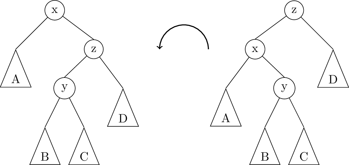
The following illustration demonstrates a left rotation on the root node, x:

In this illustration, the triangles A, B, C, D represent subtrees which might be empty (null), or they might contain 1 node, or a whole bunch of nodes. The important thing is that the subtrees don’t change, they just get moved around. In fact, there are only really two links that get changed in a rotation; they are highlighted in red in the image above.

(Well technically, we should say there are three links that get changed. The third one is the link to the root node, which used to point to node x and now points to y.)

Pseudocode for a left rotation is as follows:

Node lRotate(Node oldRoot) {    // oldRoot is node "x" in the image above.
  Node newRoot = oldRoot.right; // newRoot is node "y" in the image above.
  Node middle = newRoot.left;   // middle is the subtree B
  newRoot.left = oldRoot;
  oldRoot.right = middle;
  return newRoot;
}

A right rotation on the root node is exactly the opposite of a left rotation:

To implement rRotate, you just take the code for lRotate, and swap right and left!

4.3 Rebalancing

Rebalancing an AVL tree node means taking a subtree which is still in BST order (as always!), but may have balance factor +2 or -2, and performing some tree rotations so that that subtree is AVL balanced again.

Specifically, to rebalance a node, we require that:

• The balance factor of that node is between -2 and 2
• The balance factor of all descendent nodes are between -1 and 1. (That is, the left and right children are both AVL balanced.)
• All nodes in the subtrees store their height properly. (That is how we recompute the balance factors!)

Normally, to fix a node which has balance factor -2, we do a right rotation, and to rebalance a node with balance factor +2, we do a left rotation. Easy!

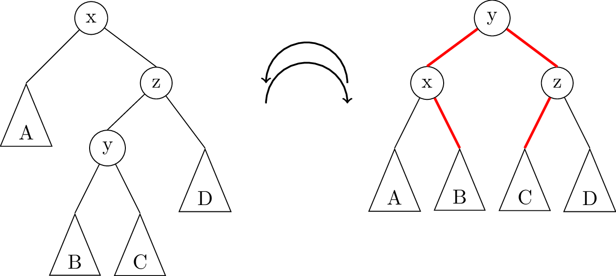
Except that this doesn’t always work. Consider the following tree, where we assume all subtrees A,B,C,D are already AVL-balanced and they all have the same height:

In the picture above, node x is ripe for rebalancing with a left rotation: x has balance factor +2, while its children are all AVL-balanced. But as we can see, a single left rotation on node x doesn’t fix anything; it just makes x unbalanced in the other direction.

The trouble here is that the “extra weight” before rotation is on the “inside” of the tree. In this case, we are doing a left rotation on x, but the node we would bring to the root, z, is already “left-leaning” with a balance factor of -1.

To fix it, we perform a double rotation. In a double rotation, you fix the “extra weight on the inside” problem by first rotating the subtree in the opposite direction of the top rotation, then doing the rotation you wanted on the top. In this case, we would first do a right rotation on node z, then a left rotation on x, to result in the following balanced tree:

Putting this all together, the logic for rebalancing a node is like this:

• If the node has balance factor -1, 0, or 1, then it is already balanced. Do nothing.
• If the balance factor is -2 then:
  • If the left child balance factor is +1, then do a left rotation on the left child first. (Double rotation case)
  • Now do a right rotation on the node itself.
• If the balance factor is +2 then:
  • If the right child balance factor is -1, then first right-rotate the right child
  • Afterwards, do a left rotate on the node itself.
• Recalculate the height of the current node based on its two children.

Don’t forget that last step! We need the height to be correct in order for future rebalancings to know the right thing to do!

4.4 Getting an element

This is no different from find or get in any other binary search tree! You just start at the root and go left/right according to what you are searching for, until you find it or hit a null node.

Remember, an AVL tree is a BST with extra rules.

4.5 Inserting or removing a node

Inserting or removing from an AVL tree starts out exactly the same as we did for binary search trees. The main idea is to always maintain the BST ordering left-right property, and never try and insert or remove nodes in the middle of the tree:

• Inserting a new node will always go as a leaf node at the bottom of the tree.
• Removing a leaf or “elbow” (one-child) node means replacing with its only child
• Removing a two-child node first swaps contents with its successor, then removes its successor below. (The successor node will never have two children.)

The tree rotations come into play after the normal BST insertion or removal takes place. Specifically, we call the rebalance() operation on every node from the insertion/removal point back up to the root of the tree. This is really easy to do with recursion - you just add the call to rebalance() after the recursive call.

4.6 Height of an AVL Tree

So far, we know that we can implement the Map ADT with an AVL tree, which is a special kind of BST which maintains a balance property at every node. And we know that the cost of get and set in a BST is \(O(height)\). If you think about it, each AVL rotation operation is \(O(1)\), and so even in an AVL tree, the get and set operations are \(O(height)\).

What makes AVL trees useful is that, unlike any old Binary Search Tree, the height of an AVL tree is guaranteed to be \(O(\log n)\), where \(n\) is the number of nodes in the tree. That’s amazing! Here’s how you prove it:

Let’s write \(N(h)\) to be the minimum number of nodes in a height-\(h\) AVL tree. Remember that we know two things about an AVL tree: its subtrees are both AVL trees, and the heights of the subtrees differ by at most 1. And since the height of the whole tree is always one more than one of the subtree heights, the balance property means that both subtrees have height at least \(h-2\).

Now since both subtrees have height at least \(h-2\), and both of them are also AVL trees, we can get a recurrence relation for the number of nodes:

\[N(h) \geq \begin{cases} 0,& h=-1 \\ 1,& h=0 \\ 1 + 2N(h-2),& h\ge 1 \end{cases}\]

This isn’t a recurrence for the running time of a recursive function, but it’s a recurrence all the same. That means that we know how to solve it! Start by expanding out a few steps:

\[\begin{align*} N(h) &\geq 1 + 2N(h-2) \\ &\geq 1 + 2 + 4N(h-4) \\ &\geq 1 + 2 + 4 + 8N(h-6) \end{align*}\]

You can probably recognize the pattern already; after \(i\) steps, it’s

\[N(h) \geq 1 + 2 + 4 + \cdots + 2^{i-1} + 2^i N(h-2i)\]

We know that the summation of powers of 2 is the next power of 2 minus 1, so that can be simplified to

\[N(h) \geq 2^i - 1 + 2^i N(h-2i)\]

Next we solve \(h-2i \le 0\) to get to the base case, giving \(i=\tfrac{h}{2}\). Plugging this back into the equation yields:

\[\begin{align*} N(h) &\geq 2^{h/2} - 1 + 2^{h/2} N(0)\\ &\geq 2^{h/2 + 1} - 1 \end{align*}\]

Hooray - we solved the recursion! But what now? Remember that \(N(h)\) was defined as the least number of nodes in a height-\(h\) AVL tree. So we basically just got an inequality relating the number of nodes \(n\) and the height \(h\) of an AVL tree:

\[n \ge 2^{h/2+1} - 1\]

Solve that inequality for \(h\) and you see that

\[h \le 2\lg(n+1) - 2\]

And wouldn’t you know it, that’s \(O(log n)\).

4.7 AVL tree runtimes

OK! So, AVL trees are guaranteed to be of \(O(\log n)\) height! Does this mean that they’re necessarily fast? Well, get(k) is unchanged from normal BSTs, so get(k) is \(O(\log n)\). That’s a great improvement over a normal BST! What about put?

Well, your pseudocode for an insertion looks like this:

private Node put(Node n, K key, V value){
  if n is null
    return new Node(key,value)
  if key==n.key
    replace n.value with value
  else if key<n.key
    n.left=put(n.left,key,value)
  else
    n.right=put(n.right,key,value)
  //so far, it's just the same as a BST insert!  But now, we need to do checks
  //and fix any unbalanced nodes, as we return our way back up the tree.
  if n is unbalanced
    perform necessary rotations
    return new root of this subtree
  return n

OK, so is this fast? We know that performing a rotation is \(O(1)\), and there are at most two rotations required to fix an unbalanced node, so we have added no real extra work there. And because each AVL tree node stores its own height, the check “if n is unbalanced” is also \(O(1)\) time.

This means that, even for the complicated operations of put and remove, they are still O(height), which we now know to be \(O(\log n)\) in the worst case.

In other words: the extra balancing requirements of AVL trees give us a much better guaranteed worst-case height of \(O(\log n)\), and the extra work we have to do to maintain that balance doesn’t change the big-O cost of the othe operations.

	Unsorted Array	Sorted Array	Unsorted Linked List	Sorted Linked List	Balanced Binary Search Tree
put(k,e)	Amortized O(1)	O(n)	O(1)	O(n)	O(log n)
get(k)	O(n)	O(log n)	O(n)	O(n)	O(log n)

5 2-3-4 Trees

Our next self-balancing tree is called a 2-3-4 tree (or a B-tree of order 4), so called because nodes can have anywhere from two to four children. Regular binary search trees can’t always be perfectly balanced - that’s why AVL trees have to allow the flexibility that subtree heights can differ by at most 1.

But because 2-3-4 trees allow nodes to have 2, 3, or 4 children, they can always be perfectly balanced! In other words: in a (balanced) 2-3-4 tree, all leaf nodes are at the same level, and every non-leaf node has their full complement of children (ie, no children are null).

Nodes in a 2-3-4 tree can contain multiple pieces of data, but the rules stay similar to a binary search tree; things to the right are bigger than things to the left. The nodes look like this:

In the above image, in the 2-node, the red subtree consists of data smaller than 5, and the purple data consists of data larger than 5. In the 3-node, red data is smaller than 3, blue is between 3 and 7, and purple is larger than 7. In the 4-node, red is smaller than 3, yellow is between 3 and 5, blue is between 5 and 7, and purple is larger than 7. In summary:

• A 2-node has 1 key and 2 children.
• A 3-node has 2 keys and 3 children.
• A 4-node has 3 keys and 4 children.

In general, the number of children of any node has to be exactly 1 more than the number of keys in that node. The keys in a node go “between” the keys of each child subtree.

5.1 Splitting a 4-node

Just like rotations where the key operation to keeping an AVL tree balanced, node split operations are the key to maintaining a balanced 2-3-4 tree when we do additions. Here’s how splitting works:

• Only a 4-node can be split.
• The smallest key and the two smallest children form a new 2-node.
• The largest key and the two largest children form a second new 2-node.
• The middle key goes into the parent node (it gets “promoted”), and the new 2-nodes are new children of the parent node.

For example, given the following 4-node:

it would be split as follows:

In that image, the (x) and (z) nodes are newly-created 2-nodes, and the (y) would be inserted into the parent node. If there is no parent node, meaning that (x,y,z) was the root node before, then (y) becomes the new root node.

5.2 Adding to a 2-3-4 Tree

The algorithm for insertion is dead-simple, once you understand how to split. What makes it easy is that we follow this rule: you never insert into a 4-node. Whenever you encounter a 4-node that you might want to insert into, you split it first! Here’s an example:

Let’s first try to insert 18:

That was easy! There were no 4-nodes along the way, so no splits needed and we just put 18 in the leaf node where it belongs.

Now let’s keep going and insert 60:

See what happened? The search for 60 ended up in the 4-node (33,40,52). Since we can’t insert into a 4-node, we split that node first and promoted 40 to the top level before proceeding to insert 60 below.

Keep going: insert 79:

That time, two splits were necessary in order to do the insertion. Since we split the root node, we got a new root node (and the height of the tree increased by 1).

So how long does an insert take? Well, in the best case, all the nodes along the search path are 2-nodes or 3-nodes, so we can just add the new value to an existing leaf node. That takes \(O(\log n)\), since the height of a 2-3-4 tree is always \(O(\log n)\).

In the worst case, we have to split at every level down to the leaf. But each split is a constant-time operation, so the cost in the worst case is still \(O(\log n)\)! Therefore the cost of get or set in a 2-3-4 tree is \(O(\log n)\).

5.3 Implementing a 2-3-4 Tree

So how do we implement this? Well… you probably don’t. There’s another balanced BST called a Red-Black Tree which is equivalent to a 2-3-4 tree, but where every 2-3-4 node is turned into 1, 2, or 3 BST nodes that are either colored “red” or “black”. People tend to use red-black trees as the implementation because some of the rules for balancing are easier to implement, particularly when you want to remove something from the tree. (In the linked-to Wikipedia article, check out the section called “Analogy to B-trees of order 4”).

If you’re implementing your own balanced tree, you might want to choose to look up a Red-Black tree and do it that way. However, you are not required to know anything about them for this course.

5.4 Comparison to AVL Trees

The tallest a 2-3-4 tree would be one made up entirely of 2-nodes, making it just a binary search tree. But since 2-3-4 trees are always perfectly balanced, the height in that worst case would still be \(O(\log n)\), comparable to AVL trees. But, which is better?

This is a complicated questions, and as is often the case, the answer is “it depends.” When we compare AVL Trees and Red-Black trees, we find they are quite similar - AVL trees have stricter balancing rules to adhere to, so they are slightly shorter, and therefore can have a faster find(). It’s not clear which type of binary tree requires more rotations - it depends on the data and the order it’s added in.

A more interesting is a comparison of AVL trees and a generalization of a 2-3-4 tree called a B-tree. You can imagine adding 5-nodes to make a 2-3-4-5 tree, or, indeed, adding larger and larger nodes, until we make a B-Tree of order k, where k is the largest allowed node size. Variations on these B Trees are frequently used in databases, storing data on the hard disk. Large nodes can hold large amounts of data contiguous to each other on the hard disk, allowing for faster retrieval of ranges of data, with less hard drive searching.