This unit is our deepest investigation into the details of how interpreters and compilers work on the back-end. First we discuss garbage collection, which is how a running process handles the de-allocation of memory that is no longer going to be used by the program. Next, we start moving towards thoughts of compilers by discussing virtual machines, that directly interpret some partially-compiled bytecode from the original source. After that, we start talking about actual compilers with a look at intermediate representations that are used as some kind of language between the original source code and the target machine code. These allow the compiler to do some great optimizations and supercharge your program’s efficiency. We could easily spend an entire course on these topics, so this unit will be necessarily choosing just a few interesting aspects to look at in detail.

1 Garbage Collection

1.1 Lifetime Management

Remember that the lifetime of a variable refers to how long that variable actually stays stored in memory. The lifetime of a variable generally starts when it gets declared or defined (or when its scope is entered), but the end of lifetime can be a bit more tricky. Where do variables go to die? That’s what we’re going to look at in this unit.

Recall from Unit 6 that there are three ways variable storage can be allocated in a program: statically, on the stack, or from the heap. Statically allocated variables have a lifetime equal to the entire program execution; they never die. Stack allocation is tied to function calls, so anything allocated on the stack (such as local variables within a function) will simply be de-allocated when that function returns.

The problematic case is the third one: heap allocation. Heap-allocated variables include all Objects in Java, everything that is malloc-ed or new-ed in C++, and just about everything in Scheme. The reason for “just about everything” in Scheme is that Scheme implements lexical scoping using Frames and closures, which are not automatically destroyed when a function exits.

These heap-allocated objects definitely need to be de-allocated. Otherwise, your Java or Scheme program would just keep eating up more and more memory until it crashed. How would you like to restart your favorite application every few hours, or your whole operating system for that matter?

The first option in memory de-allocation is “make the programmer do it”. This is the approach of C and C++, where we have to use commands like free and delete to explicitly de-allocate any heap-allocated storage. This will be the fastest option, but only if it’s done correctly! Otherwise, there are two kinds of bad things that can happen:

• Memory leaks. This is what happens when some piece of memory is no longer being used by the program, but it was never de-allocated. It makes your program eat up more and more memory, even if the data that the program is actually working with is not increasing in size.
• Dangling references: This is the opposite problem, when some piece of data is “prematurely” de-allocated and then still gets accessed later. The dangling reference will probably return a segfault, or (worse!) just insert some nonsense into your running program.

Of these two, dangling references are definitely worse because they will cause a program to crash, badly. Memory leaks are bad, but actually there have been plenty of software programs written with memory leaks that people have used for years. If the leak is small enough, it will take a very long time to notice it, and even longer to find and fix it.

Associated with dangling references is another phenomenon you may encounter, a double free. This is what happens when you de-allocate some block of memory, and then try to de-allocate the same thing again. It will cause your program to crash in a most unpleasant manner.

In summary, we see that the “manual” option for garbage collection (de-allocation) is potentially the fastest, but also very error prone. Wouldn’t it be nice if someone dealt with this for you? Well, that’s called automatic garbage collection, and we’ll look at the two basic approaches for how to do it.

1.2 Reference Counting

Automatic garbage collection is all about determining the reachability of objects in memory, during run-time of any given program. Reachability simply means whether it is possible for the program to get back to that object through any chain of references from the variables that are currently in scope. If some object is not reachable, then it is impossible for that data to be used again by the program, and so we can safely de-allocate it. How to automatically (and quickly!) determine reachability is the key question.

Reference counting is the first approach to automatic garbage collection, and it is implemented by maintaining a count of how many references (or pointers) there are to each object in a running program. Anything that has 0 references to it must be unreachable, so it will be de-allocated.

More precisely, every object in a running program gets an extra storage field that stores the number of references to that object. Whenever a pointer is created, the thing it points to gets its reference count updated immediately. Whenever an object is destroyed, or a pointer is re-assigned, whatever it used to point to has its reference count decreased immediately. As soon as the reference count goes to zero, that object gets deallocated. Note that this might cause a chain of deallocations as an object gets deallocated, then the things it points to have their reference counts decrease, then they get deallocated, etc.

How about an example? Here’s a Scheme program:

(define (f x y)
  (define (g z)
    (if (<= (abs (- x z)) (abs (- y z)))
        x
        y))
  g)

(define posneg (f -1 1))

(display (posneg 21))
(display (posneg -3))
(display ((f 10 20) 18))

See if you can figure out what this program does. The function f is actually a factory that makes a function to determine whether its argument is closer to x or to y. Since posneg has x=-1 and y=1, it will determine whether its argument is positive or negative.

The following diagram shows the frames and closures that result after running this program. The numbers in green to the left of each frame are the reference counts of each frame.

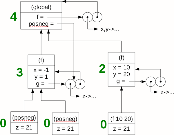
The reference counts are pretty easy to figure out; they are just the number of pointers (arrows) into each frame. The only exception is the global frame, which always gets a +1 pointer for free, to make sure it doesn’t get de-allocated.

(More generally, whatever frame represents the current scope would get the magical +1 reference count to ensure it is not de-allocated. But for our purposes, we’ll always do garbage collection from the global scope, so this isn’t an issue.)

If the Scheme interpreter had garbage collection via reference counts, then all three frames on the bottom with count 0 would be de-allocated. This would decrease the reference counts on the two frames in the middle (the frames for f) down to 1 each. So we would end with three frames kept in memory: the global frame, and both frames for f.

First, remember that garbage collection wouldn’t actually happen all at once like this; with reference counts, objects are deallocated as soon as their reference count goes to 0, so in this case, each of the bottom three frames would be deallocated as soon as that function returned.

Second, you may be wondering why we aren’t writing reference counts for the closures. The answer is that we could, but since it doesn’t work like that in your SPL interpreter in Lab 11, we’re just focusing on the reference counts for frames in these examples.

Now take a close look at the three frames that remain after the reference count-based garbage collection. See the issue? The second frame for (f) is not reachable anymore, but it will not be de-allocated because there is still something pointing to it. The real issue here is the circular reference from that frame to the closure for g and from the closure back to the frame itself. This is the essential problem with reference counting: there is the potential to undercount and leave things in memory that could be deallocated. This is actually why reference counting gets used in filesystems, because circular references are explicitly forbidden. (You can’t make a hard link on a directory.) Otherwise, if circular references can exist, and there are no other tricks or techniques, there is the potential for memory leaks with this kind of garbage collection.

1.3 Mark and Sweep

Mark and sweep is the main alternative to reference counting as a way of implementing automatic garbage collection. It is a much more aggressive strategy than reference counting, because it ensures that only the “reachable” objects will stay in memory. However, it is more costly than reference counting, as it requires the whole program to halt while the garbage collection happens.

Unsurprisingly, mark and sweep garbage collection involves two stages: mark, and sweep!

In the marking stage, the idea is to “mark” every object which is reachable from the current scope. This mark might be implemented in a variety of ways; the simplest is to add an extra boolean (maybe just implemented as a single bit) to each object in memory.

Marking begins with everything being unmarked. Beginning with a “root set” corresponding to the current scope, everything in the root set is marked, and then anything that is pointed to by some object in the root set is marked, then anything that is pointed by any of those objects is marked, etc, until there is nothing left to mark. This is usually implemented using recursion and essentially amounts to a depth-first search on the graph of objects and references in the running program. The important thing to remember is that an object gets marked before all its pointers are explored recursively; otherwise there will be an infinite loop!

The second stage is sweeping, and the idea is to deallocate every object that was not marked. In practice, what this means is going through every single object in memory, clearing the mark if it has been set, and deallocating the object if the mark is not set. This is really the “garbage collection” part of the process.

Here is a diagram with the frames and closures from the same program as above, after a mark-and-sweep operation. Starting with the global frame as the “root set”, first the two closures that the global frame points to are marked. Then, by recursion, the frame for the first call to (f) is also marked, because it is pointed to by the closure for posneg. Thus ends the recursive exploration for marking, so the objects in green are marked (and kept in memory). In the sweep stage, all the other objects (shown in red below) are deallocated.

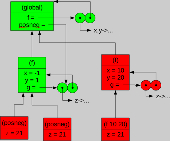
Notice that mark and sweep really gets everything; this process did not leave behind the second (unreachable) frame for (f) just because of the circular reference. But there is a price to be paid for this higher quality of garbage collection, in terms of efficiency. A mark and sweep operation can’t update as it goes along, like we can do with reference counts. Instead, performing this kind of garbage collection requires the entire program to be halted for the mark and sweep operations. This can slow down programs significantly, even if there is not much garbage to actually be collected.

1.4 Other tricks

We’ve examined the two primary approaches to automatic garbage collection: reference counts and mark-and-sweep. As is usually the case, reality gets a bit more complicated than this. Most garbage collection that happens in modern languages is some kind of variation of the above options, either to make the garbage collection more efficient, or more effective, or both. I’ll point out a few of the interesting options that get used, and you can read more about them if you want.

• Stop and copy. This is like mark and sweep, but no actual marking occurs. Instead, during the marking phase, every time we would go to mark another object, it is instead copied to a new region of memory. This continues recursively, until all of the reachable objects have been copied to the new memory region. (And of course all of their links are updated to point to each other in that new region as well.) Then the sweep stage is highly simplified: it just means de-allocating the current region in its entirety. This approach wastes some memory in copying objects, but can also be more efficient because of the simplified sweep stage and no need to store a “marked” field in each object.

• Generational garbage collection. Compiler/interpreter designers made an important observation from watching garbage collection work in practice on typical programs: most garbage is new. That is to say, most of the objects that will be de-allocated have been allocated very recently. In other words, if an object survives a few rounds of garbage collection, it’s very likely to survive the next round as well. Generational garbage collectors take this into account by dividing all objects in memory into a few levels (“generations”) based on how many garbage collections they have “survived” through. Garbage collection is performed most frequently on the objects in the first generation - the newest ones. It is performed less frequently on older objects. This drastically improves the performance of automatic garbage collectors because they don’t have to run through the entirety of a program’s memory every time. It is the approach currently used in the Java virtual machine and in DrScheme.

• Conservative garbage collection. All of the automatic garbage collection methods above require some knowledge of types at run-time. At the very least, we have to know what is a pointer and what isn’t. The trouble is, in some programs, especially if they’ve been compiled and highly optimized, there’s really no way to tell the difference between an int and a pointer - they’re both just numbers in memory. Conservative garbage collection overcomes this pitfall in a seemingly stupid way: just assume that everything is a pointer. If it points to an invalid or unavailable memory location, then forget it. If it points to a valid memory location that is being used by this program, then assume it really is a pointer and proceed accordingly. This is the approach used in some languages such as Python that interface extensively with “native” code written in C or other low-level languages that don’t store very much type information at runtime. It seems like a dumb idea, but it actually works pretty well in practice!

2 Virtual Machines

We’ve seen a few options for how automatic garbage collection can work. The question that remains is, where does it happen? In an interpreted language like SPL or Scheme, this question is easy enough to answer: the interpreter will perform automatic garbage collection as it sees fit. This is in fact what you are asked to implement in Lab 11.

In a compiled language, the question is a bit trickier. The most obvious choice is to embed the routines for automatic garbage collection within the compiled code. This works fine, but will result in “code bloat”, where suddenly every compiled program, no matter how small or simple, must contain a whole bunch of code to do garbage collection. An alternative is to use some shared library routines, but that may be difficult to accomplish depending on the language, and takes away the “stand-alone” nature of the compiled binary.

A third option is achieved when the programming language straddles these two options of interpreted versus compiled. How is this possible? With virtual machines! You should already know that going from Java source code to a program execution happens in two steps:

1. The source code is compiled into something called bytecode. Notice that this is not the same as machine code. Bytecode is specially-defined for the virtual machine for that language, and it doesn’t depend on the particular architecture you’re running on. So bytecode for a Mac is the same as bytecode for Linux or Android or Windows.
2. The bytecode is interpreted in the virtual machine. This virtual machine actually runs on the target architecture and handles the actual program execution.

In this setup, automatic garbage collection is obviously and very conveniently handled by the virtual machine itself. This gains the advantages of having some compile-time processing for optimizations and type-checking, while still maintaining a small compiled image (the bytecode), and furthermore one that can be used on any platform that has a VM!

In fact, this platform-independence of code that comes from having virtual machines is one of their great benefits. If we want our code to work on a new kind of computer, all that must be done is to implement the virtual machine for that kind of computer. And if the programming language and computer are popular enough (e.g., Java), then it’s likely someone else has already done that hard work, so your code can be used on any platform with ease. Historically, this is a big part of the reason behind Java’s popularity.

The other main benefit of virtual machines is the security that they might provide. This really has nothing to do with the rest of this unit, but it’s worth knowing. Virtual machines can be run in a “sandboxed” execution mode which restricts some privileges of the program, like blocking access to some connected devices or parts of the filesystem. While such restrictions are possible in principle at the operating system level, in practice they often do not work very effectively or very precisely, because of the simple fact that the operating system doesn’t have a way of knowing the meaning (semantics) of the code that is being executed on it. The virtual machine, by contrast, is tightly connected to the language itself and so has a better chance of determining the program’s intent, and therefore making restrictions as necessary.

3 Intermediate Representations

Modern compilers generally work in many phases of analysis, simplification, and optimization. After each stage, the code is in some intermediate representation (IR) internal to the compiler.

The initial stage of IR may be an abstract syntax tree (AST). Indeed, in interpreted languages without much optimization, the AST may be the only IR used.

The bytecode language of various virtual machines, as we just discussed, is another kind of IR. This bytecode is usually a stack-based language, where one of the main goals is to make the bytecode as small as possible while still allowing fast low-level execution. These bytecode languages are often closely tied to the features of the original source code language (e.g., Java bytecode is closely tied to the Java language).

Optimizing compilers nowadays also go through at least one more stage of IR, after the AST, looking closer to the ultimate goal of machine code while still being independent of the target architecture. The kind of IR that compilers use has different goals than ASTs or bytecode: it is designed to be easy to optimize in later steps of the compilation, rather than being targeted towards simplicity or compactness.

We will focus on some properties of an IR which is both language and machine-independent:

• Three-address code (3AC)
• Basic blocks
• Control flow graph (CFG)
• Single static assignment (SSA)

These are the properties shared by some IRs for popular modern compilers, which have the attractive property of being language-independent and machine-independent. That means that you can produce this IR from any initial programming language source code, and from this IR you can produce actual machine code for many different target architectures.

In our final double-credit lab, we will look at compiling to the IR for LLVM, the modern compiler suite behind clang and clang++. The IR properties we cover here are very similar to those found in the LLVM IR, so will be relevant to your work in that lab.

3.1 Three-address code

A three-address code, abbreviated 3AC or TAC, is a style of IR in which every instruction follows a similar format:

destination_addr = source_addr1 operation source_addr2

Some operations in 3AC have fewer than 3 addresses, but usually not more. This is quite similar to many basic machine instructions like ADD or MUL, but it’s important to emphasize that a 3AC IR is still machine-independent and will usually be simpler than a full assembly language like x86 or ARM.

Sometimes (confusingly) the instructions of a 3AC are called “quadruples”, because they really consist of four parts: the operation, the destination address, and the two (or sometimes one) source addresses.

The number of operations is usually relatively small compared to a full programming language. For example, you wouldn’t probably have a += operator to add and update a variable; instead you would have to use addition where the destination address matches the first source address.

Like assembly code, 3AC languages don’t usually have any looping or if/else blocks. Instead, you have goto operations and labels. In the LLVM IR we will use, an unconditional branch looks like

br <label>

and in a conditional branch we see the more typical 3AC structure:

br <condition_addr> <label1> <label2>

In the conditional branch, condition_addr is the address of a boolean value. If that value is 1 (i.e., true), then the code jumps to label1, and otherwise it jumps to label2.

An example is in order! Consider this simple Python code fragment to compute the smallest prime factor p of an integer n.

p = 2
while p*p <= n:
    if n % p == 0:
        break
    p += 1
if p*p > n:
    p = n
print(p)

Now let’s see how that might translate into 3AC:

    p = 2
condition:
    temp = p * p
    check = temp <= n
    br check loop afterloop
loop:
    temp = n % p
    check = temp == 0
    br check afterloop update
update:
    p = p + 1
    br condition
afterloop:
    temp = p * p
    check = n < temp
    br check if2 afterif
if2:
    p = n
    br afterif
afterif:
    # Note: this is one plausible way a library call could work,
    # assuming some special variable names arg1, arg2, etc.
    arg1 = "%d\n"
    arg2 = p
    call printf

Notice that it got quite a bit longer - that’s typical, because we have to take something that used to be on one line like if p*p > n, and break it into multiple statements. This also involves adding some new variables which didn’t exist in the original program. In this case, we added new variables temp and check as temporaries to store some intermediate computations.

3.2 Basic blocks and (the other) CFGs

A useful property of most IRs is that they make it easier for the compiler to analyze the control flow of the program. The way this is typically represented is by first breaking the program into a number of basic blocks - sequential chunks of statements with no branches. In the strictest setting (which the case for LLVM IR that we will see in lab), each basic block must start with a label and end with some control flow statement like a branch or a function call.

The example above is almost in basic block form already, except that we need to give a label to the first block and add an unconditional branch at the end of it:

initial:
    p = 2
    br condition
condition:
    temp = p * p
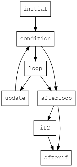
    # ... the rest is the same

Once the program is broken into basic blocks, we can generate the control flow graph (CFG) showing possible execution paths in the program between the basic blocks. Specifically, each node in the CFG is a basic block, indicated by its label, and each directed edge represents a possible execution path from the end of that basic block to another one.

(Note: CFG is now an overloaded term in this class, because it also stands for Context-Free Grammar in the context of parsing. Hopefully the context (haha) will make the distinction clear.)

Here is the CFG for the prime factor program above:

3.3 SSA

The final aspect of the modern IRs (including the LLVM IR) that we will look at is called static single assignment, or SSA. This is a restriction in how variable or register names are assigned in the IR which makes many later compiler optimizations much easier to perform. Interestingly, SSA is very closely related to the concept of referential transparency that we learned from functional programming.

Here’s the formal definition:

A program is in SSA form if every variable in the program is assigned only once.

That is, any name can appear on the left-hand side of an assignment only once in the program. It can appear many times on the right-hand side (after the assignment!), but only once on the left-hand side. This model is also called write once, read many.

Let’s recall our running example of the prime factor finding program, in 3AC form:

initial:
    p = 2
    br condition
condition:
    temp = p * p
    check = temp <= n
    br check loop afterloop
loop:
    temp = n % p
    check = temp == 0
    br check afterloop update
update:
    p = p + 1
    br condition
afterloop:
    temp = p * p
    check = n < temp
    br check if2 afterif
if2:
    p = n
    br afterif
afterif:
    # Note: this is one plausible way a library call could work,
    # assuming some special variable names arg1, arg2, etc.
    arg1 = "%d\n"
    arg2 = p
    call printf

This is currently not in SSA form, because the variables p, temp, and check are reassigned in a few places.

The usual fix is to replace each reassignment with a new variable name, so that they never get reused and we have good ol SSA form back again. We’ll replace each assignment of p with p1, p2, etc., and change each subsequent usage of temp and check to t1, t2, etc.:

initial:
    p1 = 2
    br condition
condition:
    t1 = p * p  ## PROBLEM
    t2 = t1 <= n
    br t2 loop afterloop
loop:
    t3 = n % p  ## PROBLEM
    t4 = temp == 0
    br t4 afterloop update
update:
    p2 = p + 1  ## PROBLEM
    br condition
afterloop:
    t5 = p * p  ## PROBLEM
    t6 = n < t5
    br t6 if2 afterif
if2:
    p3 = n
    br afterif
afterif:
    arg1 = "%d\n"
    arg2 = p    ## PROBLEM
    call printf

Great! This now follows the SSA form wherein each variable name is assigned only once, except there are some problems very subtly identified in the code above. Take a second to see if you can figure out what the trouble is here.

The problem is, now that we’ve changed all the reassignments of the original variable p to p1, p2, and p3, how do we know what each usage of p refers to on the right-hand side? Take for example the first problem:

t1 = p * p

You might be tempted to say that p here should be p1, from the initial block. And sure, that’s what p will be the first time around. But the next time the condition block is executed, it’s not coming from the initial block but rather from the update block, so at that point p should be p2.

In other words, the value p in this line could be coming either from p1 or p2, depending on where the program actually is in its execution. This was not a problem with the temp and check variables that we replaced with t1, t2, and so on, because their uses were within the same basic block where the variable was set, so there wasn’t any question.

But p is essentially acting as a conduit for communication between the basic blocks, being set in one block and accessed in another.

Now, there are two basic ways to solve this. The “easy way” is to use memory: for any variable like p which has some ambiguous uses, we simply store p into memory (on the stack), and load its value from memory each time it is used. Then we only need to save the address of p within the variables of the program, and even though p may be changing repeatedly, that address never changes, so the rules of SSA are not violated. In fact, this is the approach we will take in our LLVM IR lab.

But using memory this way is very costly in terms of computing time. Each load or store from RAM (or even cache) is hundreds or thousands of times slower than reading from a CPU register. So we would really like to keep these values as variables in our 3AC code, if possible, to allow the later stages of compilation to potentially store them in CPU registers and make the program as fast as possible.

The solution to this, the “hard way”, is to use what is called a phi function, written usually with the actual Greek letter \(\phi\). A phi function is used exactly in cases where the value of a variable in some basic block of the program could come from two or more different assignments, depending on the control flow at run-time. It just means adding one more assignment to the result of the \(\phi\) function, and the arguments to the phi function are the different possible variables whose value we want to take, depending on which variable’s basic block was most recently executed.

I know - that description of the phi function seems convoluted. That’s what makes this the “hard way”! But it’s how actual compilers work, and it’s not too hard to understand once we see some examples. For the case of the assignment t1 = p * p in our running example, we would replace this with

p4 = phi(p1, p2)  # gets p1 or p2 depending on control flow
t1 = p4 * p4    # Now we can use p4 multiple times in SSA form

Applying this idea throughout the program yields this complete description of our prime factor finding code, in proper SSA form:

initial:
    p1 = 2
    br condition
condition:
    p4 = phi(p1, p2)
    t1 = p4 * p4
    t2 = t1 <= n
    br t2 loop afterloop
loop:
    t3 = n % p4
    t4 = t3 == 0
    br t4 afterloop update
update:
    p2 = p4 + 1
    br condition
afterloop:
    t5 = p4 * p4
    t6 = n < t5
    br t6 if2 afterif
if2:
    p3 = n
    br afterif
afterif:
    p5 = phi(p3, p4)
    arg1 = "%d\n"
    arg2 = p5
    call printf

Ultimately, we needed only two phi functions to get this program working. How did we figure this out - when to use a phi function and when not to, or which version of p to use in each right-hand side?

Generally, this is what you have to do to figure out what any given variable reference should be replaced with in SSA form:

1. If the variable was set earlier in the same basic block, use that name. For example:

   y = 7 * 3
   y = y + 1
   temp = y < 10

   becomes simply

   y1 = 7 * 3
   y2 = y1 + 1    # y1 is the most recent defn in the same basic block
   temp = y2 < 10 # y2 is the most recent defn in the same basic block

2. If the variable was not set earlier in the same basic block, then trace backwards all possible paths in the control flow graph, moving backwards until we find the most recent setting of the variable in each path that could have reached this basic block.

   If all paths reach the same basic block where the variable was most recently set, use that variable name. For example:

   one:
       x = 5
       x = x - 3
       br x two three
   two:
       y = x * 10
       br three
   three:
       y = x + 20

   becomes

   one:
       x1 = 5
       x2 = x1 - 3     # same basic block reference
       br x2 two three # same basic block reference
   two:
       y1 = x2 * 10    # x most recently set in block one
       br three
   three:
       y2 = x2 + 20    # x most recently set in block one

3. Finally, if cases (1) and (2) both fail, then we need to have a phi funciton. Tracing backwards through the CFG, we find all basic blocks along execution paths where the variable could have been most recently set. Then we make a new variable and set it to phi of all of those possible variable values. For example, slightly changing the previous situation:

   one:
       x = 5
       x = x - 3
       br x two three
   two:
       x = x * 10
       br three
   three:
       x = x + 20

   becomes

   one:
       x1 = 5
       x2 = x1 - 3     # same basic block reference
       br x2 two three # same basic block reference
   two:
       x3 = x2 * 10    # x most recently set in block one
       br three
   three:
       x4 = phi(x2, x3)  # x could come from block one or two
       y2 = x4 + 20    # now we use x4

4 Optimizations

At this point, you should be asking “WHY!!!” Why did we do all this work to convert to the 3AC SSA Intermediate Representation and draw the CFG?

The main answer is that this representation makes it much easier for the compiler to perform code optimizations in later steps. Some examples of these optimizations are:

• Constant propagation
• Common subexpression elimination
• Dead code elimination
• Code motion
• Function inlining
• Loop unrolling
• Strength reduction
• Register allocation

Depending on timing, we may have a chance to look at a few of these in more detail. Expect this section of the notes to be expanded.