1 Dijkstra's Algorithm

BFS works great at finding shortest paths if we assume that all edges are equal, because it minimizes the number of "hops" from the starting point to any destination. But in a weighted graph, we care about the total sum of the weights along any candidate path, and want to miminize that value rather than the number of hops. In other words, it's OK to take more turns in your driving directions, as long as the total time is less.

Consider the following graph. Here, the vertices may be intersections, and the edges may be roads, with expected time to travel as the weights.

Let's consider the problem of finding the fastest route from vertex A to vertex H. A BFS would find us a path with the minimum number of hops, perhaps A - B - G - H. This path "looks" shortest, but it has total length \(5+17+15 = 37\) in the graph. There is definitely a shorter way!

The good news is that we only really have to change one thing to adapt our BFS to work with weighted graphs like this one. Instead of the fringe being a regular old queue, we will instead have a priority queue, which removes vertices according to which one has the shortest path from the starting vertex. Since we want the path with smallest weight, we will have a minimum priority queue.

Each entry in the fringe will be a vertex name, plus two extra pieces of information: the parent node, and the path length. We'll write these as a tuple; for example (C, B, 15) means "the path to C that goes through B has length 15".

Besides the fringe data structure, we also have to keep track of which nodes have been "visited", and what is the "parent" of each visited node, just like with BFS. Both of these can be maps; probably the same kind of map (either balanced tree or hashtable) that stores the vertices of the graph itself.

OK, let's get back to our example from above, and run Dijkstra's algorithm to find the shortest path from A to H. You might want to open that graph up in a new tab or print it out so you can follow along.

To run through this example, we'll look at the "state" of our three data structures visited, parents, and fringe, at each step along the way. Here's the initial state:

visited:
parents:
fringe: (A, null, 0)

1. Remove (A, null, 0) from the fringe.
   We mark vertex A as visited and set its parent.
   Then we add 2 new fringe entries for each of A's neighbors.
   

   visited: A
   parents: A->null
   fringe: (B,A,5), (C,A,7)

2. Remove (B, A, 5) from the fringe.
   Vertex B gets "visited", its parent is set to A, and its 4 neighbors are added to the fringe.
   

   visited: A, B
   parents: A->null, B->A
   fringe: (C,A,7), (A,B,10), (C,B,15), (D,B,9), (G,B,22)

   Notice: I'm not writing the fringe in order. It's a minimum priority queue, so things will be removed according to the shortest distance first; but the actual order will depend on what data structure gets used, e.g., a heap.
   Also notice: The distances (priorities) stored with each node in the fringe correspond to the total path length, not just the last edge length. Since the distance to the current node B is 5, the distances to B's neighbors A, C, D, G are 5+5, 5+10, 5+4, and 5+17.
3. Remove (C, A, 7) from the fringe.
   Vertex C gets visited, its parent is A, and its 4 neighbors go in the fringe.

   visited: A, B, C
   parents: A->null, B->A, C->A
   fringe: (A,B,10), (C,B,15), (D,B,9), (G,B,22), (A,C,14), (B,C,17), 
           (D,C,10), (E,C,22)

4. Remove (D, B, 9) from the fringe.
   Notice: This vertex is removed next because it's a min-priority queue.
   Vertex D gets visited, its parent is B, and its 3 neighbors go in the fringe.

   visited: A, B, C, D
   parents: A->null, B->A, C->A, D->B
   fringe: (A,B,10), (C,B,15), (G,B,22), (A,C,14), (B,C,17), (D,C,10),
           (E,C,22), (B,D,13), (C,D,12), (E,D,10)

5. Remove (A, B, 10) from the fringe.
   Nothing happens because A is already visited.

   visited: A, B, C, D
   parents: A->null, B->A, C->A, D->B
   fringe: (C,B,15), (G,B,22), (A,C,14), (B,C,17), (D,C,10), (E,C,22)
           (B,D,13), (C,D,12), (E,D,10)

6. Remove (D, C, 10) from the fringe.
   Nothing happens because D is already visited.

   visited: A, B, C, D
   parents: A->null, B->A, C->A, D->B
   fringe: (C,B,15), (G,B,22), (A,C,14), (B,C,17), (E,C,22), (B,D,13),
           (C,D,12), (E,D,10)

7. Remove (E, D, 10) from the fringe.
   Vertex E gets visited, its parent is D, and its 3 neighbors go in the fringe.

   visited: A, B, C, D, E
   parents: A->null, B->A, C->A, D->B, E->D
   fringe: (C,B,15), (G,B,22), (A,C,14), (B,C,17), (E,C,22), (B,D,13),
           (C,D,12), (C,E,25), (D,E,11), (F,E,13)

8. Remove (D, E, 11), then (C, D, 12), then (B, D, 13), from the fringe.
   Nothing happens because E, C, and B are visited already.

   fringe: (C,B,15), (G,B,22), (A,C,14), (B,C,17), (E,C,22), (C,E,25),
           (F,E,13)

9. Remove (F, E, 13) from the fringe.
   Vertex F gets visited, its parent is E, and its 2 neighbors go in the fringe.

   visited: A, B, C, D, E, F
   parents: A->null, B->A, C->A, D->B, E->D, F->E
   fringe: (C,B,15), (G,B,22), (A,C,14), (B,C,17), (E,C,22), (C,E,25),
           (E,F,16), (G,F,15)

10. Remove (A, C, 14), then (C, B, 15), from the fringe.
    Nothing happens because A and C are visited already.

    fringe: (G,B,22), (B,C,17), (E,C,22), (C,E,25), (E,F,16), (G,F,15)

11. Remove (G, F, 15) from the fringe.
    Vertex G gets visited, its parent is F, and its 4 neighbors go in the fringe.

    visited: A, B, C, D, E, F, G
    parents: A->null, B->A, C->A, D->B, E->D, F->E, G->F
    fringe: (G,B,22), (B,C,17), (E,C,22), (C,E,25), (E,F,16), (B,G,32),
            (F,G,17), (H,G,30), (I,G,19)

12. Remove (E, F, 16), then (B, C, 17), then (F, G, 17), from the fringe.
    Nothing happens because E, B, and F are visited already.

    fringe: (G,B,22), (E,C,22), (C,E,25), (B,G,32), (H,G,30), (I,G,19)

13. Remove (I, G, 19) from the fringe.
    Vertex I gets visited, its parent is G, and its 2 neighbors go in the fringe.

    visited: A, B, C, D, E, F, G, I
    parents: A->null, B->A, C->A, D->B, E->D, F->E, G->F, I->G
    fringe: (G,B,22), (E,C,22), (C,E,25), (B,G,32), (H,G,30), (G,I,23),
            (H,I,21)

14. Remove (H, I, 21) from the fringe.
    Vertex H gets visited, its parent is I.

    visited: A, B, C, D, E, F, G, I, H
    parents: A->null, B->A, C->A, D->B, E->D, F->E, G->F, I->G, H->I

    We can safely stop the search here because all the nodes have been visited. Of course, it would be fine to add the neighbors of H to the fringe and then remove everything; nothing would happen because everything is already visited.

Hooray! We did it! We found the shortest paths from A to H, which can be retraced by following the parent pointers backwards: H-I-G-F-E-D-B-A. This path has many hops, but the shortest possible total length of 21.

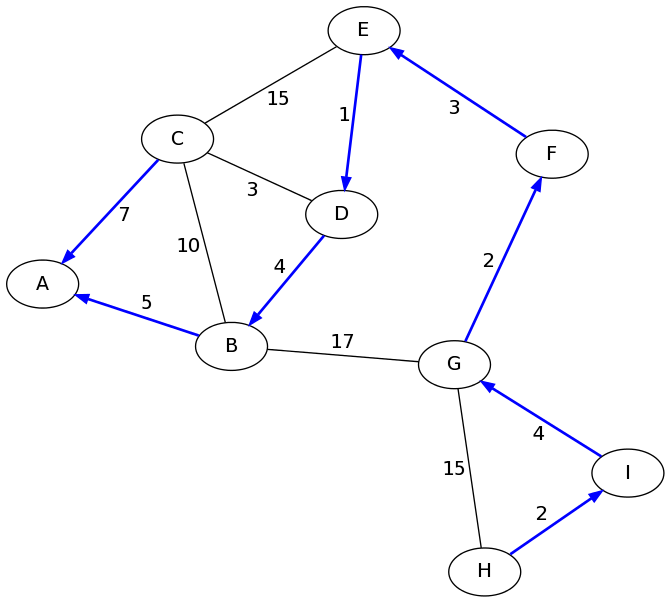
In fact, we have found all of the shortest paths from A. The parent pointers encode a tree that gives the fastest path from A to any other node in the graph. Here they are drawn in blue:

2 Dijkstra's Runtime

Here's some pseudocode for the algorithm we just learned:

1
2
3
4
5
6
7
8
9
10

function dijkstra(G, start):
    initialize fringe, parents, visited
    add (start, null, 0) to fringe
    while fringe is not empty:
        (u, par, len) = fringe.removeMin()
        if u is not visited:
            mark u as visited
            set parent of u to par
            for each edge (u,v,w) in G.neighbors(u):
                add (v, u, len+w) to fringe

Actually, if you remove the stuff about the weights and priorities, you could use exactly the same pseudocode for DFS or BFS, depending only on the data structure of fringe.

How long does Dijkstra's take? Well, it's going to depend on what data structures we use for the graph and for the priority queue. Let's go through each of the important (i.e., potentially most costly) steps in the algorithm:

• Calling removeMin() on line 5:
  The number of times this happends depends on the maximum size of the fringe. Unless we do something fancy, the fringe size is at most \(m\), so the removeMin() method gets called at most \(m\) times.
• Calling neighbors() on line 9:
  This happens once each time a node is visited, so it happens at most \(n\) times in total.
• Adding to the fringe on line 10:
  This happens once for each outgoing edge of each node, which means \(m\) times total.

So to figure out the running time for Dijkstra's, we have to fill in the blanks in the following formula: \((\text{fringe size})\times(\text{removeMin cost}) + n\times(\text{neighbors cost}) + m\times(\text{fringe insert cost}) \)

For example, if the graph is implemented with a hashtable and an adjacency list, and the fringe is a heap, the total cost is \(O(m\log m + n + m\log m) = O(n + m\log n).\) (Note that we can say \(\log m \in O(\log n)\) since \(m\) is \(O(n^2)\) for any graph.)

That's pretty good! Remember that the best we can hope for in any graph algorithm is \(O(n+m)\), so \(O(n+m\log n)\) is not too far off from the optimal.

What about another data structure for the priority queue? We should consider the "simple" choices like a sorted array or an unsorted linked list. Most of the time, those simple options aren't better than the "fancy" option (i.e., the heap). But that's not the case this time. If we use an unsorted array for the priority queue, and eliminate duplicates in the fringe so that the fringe size is never greater than \(n\), the total cost is \(O(n^2 + n\times(\text{neighbors cost}) + m) = O(n^2)\).

(To see why that's true, remember first that inserting in an unsorted array is \(O(1)\), whereas removing the smallest item is \(O(n)\). Second, the cost of neighbors() for any graph data structure is never more than \(O(n)\). Third, since the number of edges in any graph is \(O(n^2)\), you can simplify \(O(n^2 + m)\) to just \(O(n^2)\).)

What all this means is that if we use the a certain graph data structure (adjacency list with hashtable) and a heap, the running time is \(O(n + m\log n)\). But if we use ANY graph data structure with an unsorted array, the running time is \(O(n^2)\). We can't say for sure which option is better; if \(m\) is closer to \(n\) (i.e., a sparse graph), then the \(O(n + m\log n)\) would be smaller. But if \(m\) is closer to \(n^2\) (i.e., a dense graph), then \(O(n^2)\) is a better running time.

As always, it's more important that you are able to use the procedure above to decide the running time of Dijkstra's algorithm for any combination of data structures, rather than memorizing the running time in a few particular instances.