Unit 6: Sets and Maps
Credit: Gavin Taylor for the original version of these notes.
In this unit, we're going to learn why we've been learning about Binary Search Trees, and how they actually get used. We'll start with the two primary ADTs that utilize trees, Set and Map, which also happen to be two of the most important ADTs in just about any programming language. Then we'll look at ways of keeping trees balanced: AVL trees and B-trees.
Beginning of Class 16
1 Sets
It's time for two new ADTs, which are implemented very similar to each other: the Set and the Map. Sets are the simpler of the two - essentially, it keeps track of what is, and is not, in the Set. It is required that elements in the set be somehow sortable, so they can be organized and found easily.
The operations of a Set are:
- insert(e): Insert element e into the Set.
- contains(e): Returns True if e is in the Set, and False if it is not.
- size(): Returns the number of unique elements that have been inserted into the set.
2 Maps
Maps differ from Sets in that every piece of data in a Map has two parts: a key and a value. We find the value by searching for the key. For example, a dictionary is a map: we look up the word (the key), and get the definition (the value).
A phone book is a Map too: we look up the name, and get the phone number and address. The important thing is that the keys be sortable (like numbers, or strings), so that we can be smart about storing them.
Suppose we were interested in creating a system to look up a mid's grades, which wasn't as terrible as MIDS. First, you might make a class that can contain all of a single student's grades (we'll call it Grades, because we're creative). Then, you want it to be searchable by alpha.
The operations of a Map are:
get(key): Returns the value associated with the given key, orNoneif it's not in the map.set(key, value): Inserts a new key-value pair into the map, or changes the value associated with the given key if it's already in the map.size(): Returns the number of distinct keys that are stored in the map.
You may be wondering about a few things here. First, why are we using
None as a special "sentinel" value to indicate something is not
found in the map? Isn't that bad style? Well maybe it is, but this is how
some of Java's built-in methods behave, and it allows us to make the Map
interface much simpler and avoid having to deal with too many exceptions.
(The only downside is that you are not allowed to store None values in a map.)
You may also be wondering why there's no remove method. Well,
to remove something, you just set its value to None! The underlying
Map implementation can either choose to actually remove that part of the
data structure in that case, or it could just store None as the
value and no one would be the wiser!
In general, in this class, we're going to avoid talking about how removal from
Maps works, not because it can't be done, but because it's not strictly
necessary and this way we can cover a greater variety of data structures.
The same applies to removing things from a set.
3 Implementation with the data structures we know
We're going to spend a lot of time on these ADTs, implementing them with
new data structures. For now, a set/map can be implemented with an array
(either in sorted order by key, or unsorted), a linked list (again, either
sorted by key, or unsorted), or Binary Search Tree (organized by key). Note
that a Node in a LL or BST will contain a single data field for a Set, but two
data fields (key and value) for a Map. To implement a Map with an array, you
would need to combine the key and value together into a single object, like
the one below. (Alternatively, you could also use Python's tuple type
for the same purpose.)
1 2 3 4 | class KeyValuePair: def __init__(self, key, value): self.key = key self.value = value |
How would you implement these methods for each of these data structures?
| insert(k,v)/insert(e) | get(k)/contains(e) | |
|---|---|---|
| Unsorted array | O(1) (amortized) | O(n) |
| Sorted array | O(n) | O(log(n)) |
| Unsorted Linked List | O(1) | O(n) |
| Sorted Linked List | O(n) | O(n) |
| Binary Search Trees | O(height) | O(height) |
For now, we know that the height of a tree is somewhere between log(n) and n. If only we had a way to guarantee the tree would be balanced! If only...
Beginning of Class 17
4 AVL Trees
AVL Trees
We're going to learn about two types of self-balancing trees in this class, defined as "trees that always meet some definition of balanced." There's a wide variety of these, and I think they're pretty cool.
AVL Trees define "balanced" as "the heights of the subtrees of any node can differ by at most one." Note, this is NOT the same as "the tree is as short as possible." For example, consider this tree:
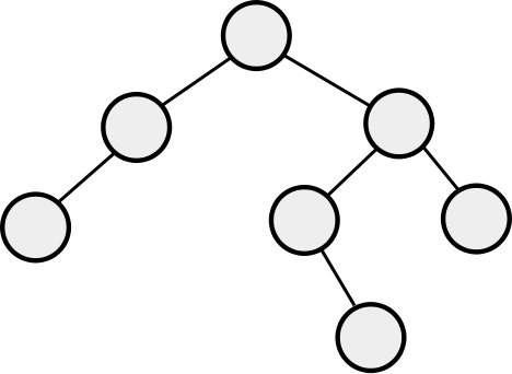
This tree is NOT complete (meaning totally filled in). However, by the definition of AVL trees, it IS balanced. The height of an AVL tree is still \(O(\log(n))\).
Rotations
AVL trees keep themselves balanced by performing rotations. A tree rotation is a way of rearranging the nodes of a BST that will change the height, but will NOT change the order. That's really important - the nodes in a BST are always in order, before and after every rotation operation. All that we change is the levels of some of the nodes to fix up the height.
The following illustration demonstrates a left rotation on the root node, x:
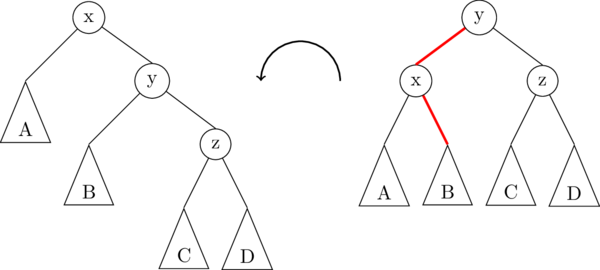
In this illustration, the triangles A, B, C, D represent subtrees which might be empty (null), or they might contain 1 node, or a whole bunch of nodes. The important thing is that the subtrees don't change, they just get moved around. In fact, there are only really two links that get changed in a right rotation; they are highlighted in red in the image above.
Pseudocode for a left rotation is as follows:
1 2 3 4 5 6 | def lrotate(oldroot): # oldroot is node "x" in the image above newroot = oldroot.right # newroot is node "y" in the image above middle = newroot.left # middle is the subtree B newroot.left = oldroot # make the connection from "y" to "x" oldroot.right = middle # make the connection from "x" to "B" return newroot |
A right rotation on the root node is exactly the opposite of a left rotation:
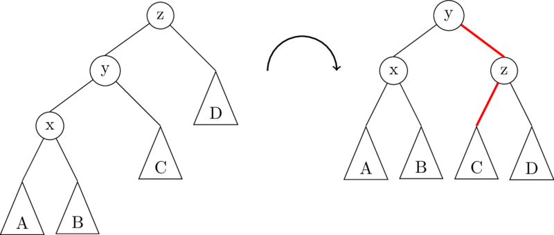
To implement rRotate, you just take the code for lRotate, and swap right and left!
Adding to an AVL tree
The idea that makes AVL trees possible to quickly implement is that nodes are modified to include the height of the subtree rooted at that node. An empty tree (null) has a height of -1, leaves have a height of 0, and any other node \(u\) has a height of \(1 + \max(u.left.height, u.right.height)\).
We also define balance, where balance = n.right.height-n.left.height.
If, at any point, balance becomes -2 or 2, we must perform at least one rotation to rebalance the tree. There are four cases to consider:
(balance(uu) == 2 && balance(uu.right) >= 0) Left rotate at the root.
(balance(uu) == 2 && balance(uu.right) == -1) Right rotate at the right subtree, then left rotate at the root. (This is called a "double rotation").
The other two cases are the mirror images of the above two.
Getting an element of an AVL Tree
This is no different from find or get in any other binary search tree!
Beginning of Class 18
Beginning of Class 19
5 B-trees
Our next self-balancing tree is called a B Tree. B Trees are different from AVL trees in that they are not binary. The branching factor of the tree (which, remember, is hte maximum number of children a node can have), is known as the degree of the B Tree. So, a B Tree of degree 4 can have up to four children.
Each type of self-balancing tree has its own rules for when a tree is balanced. A B tree is balanced when:
- All leaves have equal depth.
- If a node has ANY children, it has ALL possible children.
Nodes in a B Tree can contain multiple pieces of data, but the rules stay similar to a binary search tree; things to the right are bigger than things to the left. The nodes in a B Tree of degree 4 look like this:
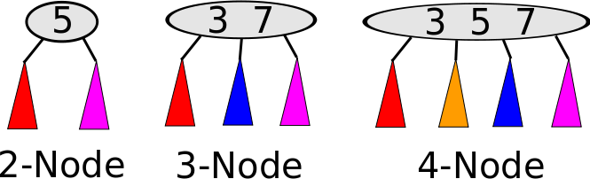
In the above image, in the 2-node, the red subtree consists of data smaller than 5, and the purple data consists of data larger than 5. In the 3-node, red data is smaller than 3, blue is between 3 and 7, and purple is larger than 7. In the 4-node, red is smaller than 3, yellow is between 3 and 5, blue is between 5 and 7, and purple is larger than 7.
Adding to a B Tree
Consider the following example B-tree where each node has a capacity of 3.

The algorithm for insertion is pretty simple. First, navigate to the appropriate leaf. Does the leaf have room for another datum? If yes, add it. In the following image, we add 18 to the tree above.

But what do we do if there isn't room? Promote the middle element to the level above, and split the node in half, like if we subsequently add 60:

Note that this process could cascade up the tree. See if you can figure out what would happen above if we inserted 80 next.
So how long does an insert take? Well, in the best case, we go all the way down to a leaf, find that there is room, and add it. That's O(log n). In the worst case, we do that log(n) work, and discover there isn't room. So, we have to do a promotion. The maximum number of promotions we'll need to do is log(n). So, the big-O of an insert with a B Tree is O(log n).
Comparison to AVL Tree
The tallest B Tree is made entirely of 2-nodes, making it a complete binary tree. This should make it clear that it's of logarithmic height, comparable to AVL trees. But, which is better?
As is often the case, the answer is "it depends." In this case, it depends on something a little bit different than in the past. We can't say that one has a better Big-O than the other, because both are \(O(\log(n))\).
Suppose the degree of your B Tree is really big, maybe even in the hundreds. Well, storing a single node may be more difficult, because it's bigger. However, when you're looking for which child to traverse to, you can do binary search on an array, which is considerably faster (not in the Big-O sense, but in the "smaller coefficient" sense) than following pointers down a tree.
We'll expand on this idea in the next lecture.
Beginning of Class 20
6 B+ Trees
The most common variant of a B Tree is known as a B+ tree. This is only slightly different from B Trees as we have learned them so far, but they are targeted at a very specific purpose: databases.
Suppose we have lots and lots of data, like in the area of billions of key-value pairs, which we would like to access quickly. So far, all of our assumptions have been based around the fact that a ``calculation" is close enough in time to every other calculation that we don't care about one or the other. In real life, this is not always the case. For example, querying a remote machine is MUCH slower than doing many calculations on the same machine. Similarly, and most relevantly, doing a calculation on data in memory is much, much faster than doing the same calculation on data which is on the hard drive, because accessing data on the hard drive actually involves moving parts (turning the platters and moving the read head).
If we have a very large amount of data, and any individual datum is only accessed occasionally, it is impossible to load all that data into memory; at some point, you're going to have to go read off the hard drive. The goal of a B+ tree is to minimize the number of hard drive seeks.
Why an AVL is a bad choice
If you had this much data, a big chunk of the top of the tree could fit into memory. However, with each layer having twice as many nodes as the layer above, nearly all nodes would have to be on the hard drive. Additionally, with each comparison, the hard drive would have to seek to the next node's location on the hard disk, which takes quite a bit of time.
Well, what if for any two layers of nodes, consisting of a parent and two children, we combined them into a single node with four children? To get to that node requires a single hard drive seek, where we could make two layer's worth of comparisons without moving the hard drive again. This is exactly the idea of the B Tree: more key-value pairs in one location leads to fewer hard drive seeks.
Why vanilla B Trees still aren't good enough
So now, minimizing hard drive accesses consists of getting as many of the top layers into memory as possible. A good way to do this is to remove having key-value pairs in the internal nodes, and merely reproducing the first key of a node in the parent node; this way you can store many more keys in the top few levels. For example:
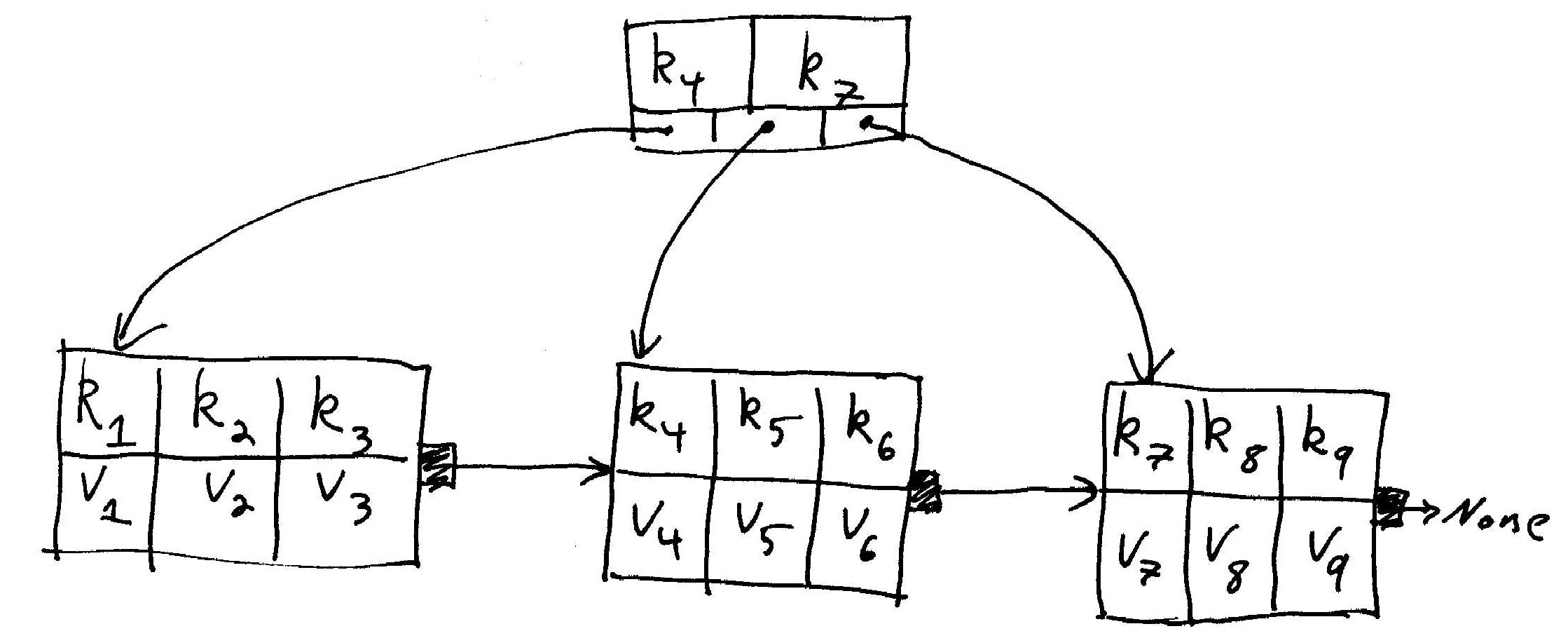
In the above picture, \(k_*\) are the keys, and \(v_*\) are the accompanying values. \(k_4\), rather than having its value stored in the upper node, instead is merely reproduced in the upper node, so as to take up less space.
But wait... there's more!
What's with the arrows between the leaves? Many database queries are along the lines of "give me every value associated with a key within the range (some key-some other key)." This is why leaves are large: the hard drive needs to seek to the first element of the block (slow), but then can read off each of these consecutive values one after another (fast), since they are physically right next to each other on disk. But what if the range extends past the end of a leaf? Well, here, each leaf contains a pointer to the next leaf, like a linked list. This allows the hard drive to move to the next block without having to re-navigate the tree.
So to summarize: B Trees, plus keeping all values in the leaves, plus pointers between the leaves, gives you a B+ Tree.