Unit 2: Big O
Credit: Gavin Taylor for the original version of these notes.
Beginning of Class 3
1 Comparing algorithms
Why do we care about all this?
Most of you carry around (the same) large black backpack all day. Think about what's in there, and where it is. Your decisions on what to put in there and where to put it all were governed by a few tradeoffs. Are commonly-used things easy to reach? Is the backpack small and easy to carry? Is it easy to find everything in there? Do you really need all that stuff every day?
Organizing data in a computer is no different; we have to be able to make decisions on how to store data based on understanding these tradeoffs. How much space does this organization take? Is the operation I want to perform fast? Can another programmer understand what the heck is going on here?
As a result, we have to start with intelligent ways of discussing these tradeoffs. This is called algorithm analysis and it's a big piece of what you're going to learn about in this class.
In order to measure how well we store our data, we have to measure the effect that data storage has on our algorithms. So, how do we know our algorithm is any good? First off, because it works - it computes what we want it to compute, for all (or nearly all) cases. At some level getting working algorithms is called programming, and at another it's an abstract formal topic called program correctness. But what we mostly will talk about here is if we have two algorithms, which is better?
So, why should we prefer one algorithm over another? As we talked about, this could be speed, memory usage, or ease of implementation. All three are important, but we're going to focus on the first two in this course, because they are the easiest to measure. We'll start off talking about time because it is easier to explain - once you get that, the same applies to space. Note that sometimes (often) space is the bigger concern.
We want the algorithm that takes less time. As soon as we talk about "more" or "less", we need to count something. What should we count? Seconds (or minutes) seems an obvious choice, but that's problematic. Real time varies upon conditions (like the computer, or the specific implementation, or what else the computer is working on).
Motivating example: primality checking
Here are two different algorithms that can be used to
determine whether a given number n is prime, meaning
its only factors are 1 and itself.
|
|
Now, you definitely do not need to understand exactly why these algorithms work in
complete detail! But you should observe that they both start by doing some simple checks,
and then they both have some loops where they do a bunch of divisibility checks using the
modulus % operator.
As it turns out, finding large prime numbers is really, really important for almost all of modern-day cryptography. So this problem really matters for cyber security!
Now - even without knowing exactly why they are correct - which of these algorithms would you predict would be faster? More important than the answer to that question, is the thought process behind what it even means to say one is "faster" than the other. Faster in what circumstance? On what computer?
One good answer to the above question is to just try running them both on a few
numbers. We can use the time.clock() funciton in Python to get really accurate CPU
timings. Here's what it gives for a few values of \(n\).
| \(n\) | is_prime1 time in ms | is_prime2 time in ms |
| 20011 | 0.0050 | 0.1760 |
| 110017 | 0.0120 | 0.2200 |
| 200003 | 0.0150 | 0.2050 |
| 290011 | 0.0180 | 0.2240 |
| 380041 | 0.0210 | 0.2300 |
| 470021 | 0.0240 | 0.2650 |
| 560017 | 0.0260 | 0.2400 |
| 650011 | 0.0280 | 0.2380 |
| 740011 | 0.0300 | 0.2310 |
| 830003 | 0.0320 | 0.2280 |
| 920011 | 0.0340 | 0.2260 |
And here's that same data in a figure. The blue dots are the times for
is_prime1, and the red triangles are is_prime2.
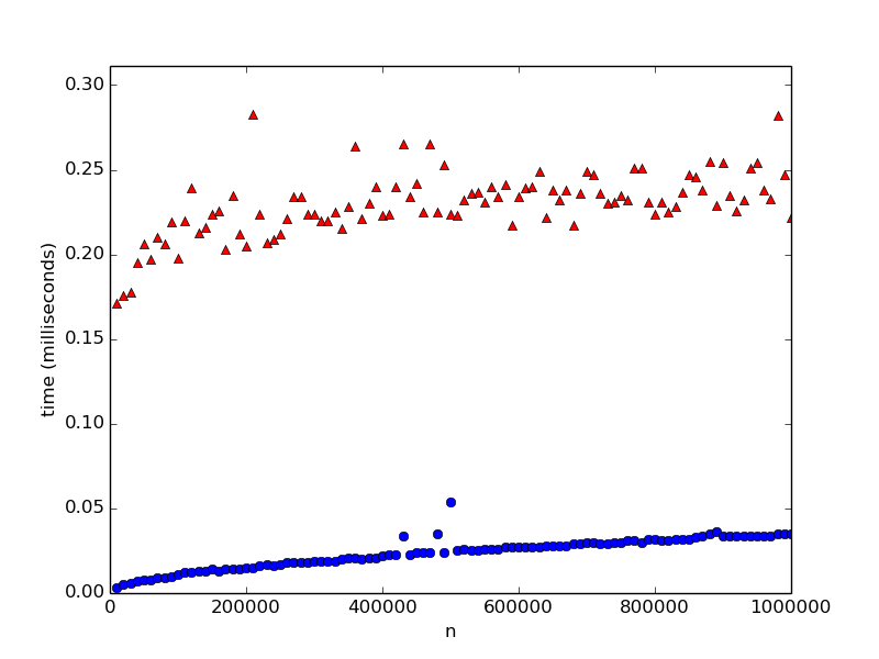
Now what do you think? Which one is faster? Are you sure? What if we test on some larger numbers, i.e. stretch this graph out further to the right? Here's one where \(n\) goes to about 1 billion:
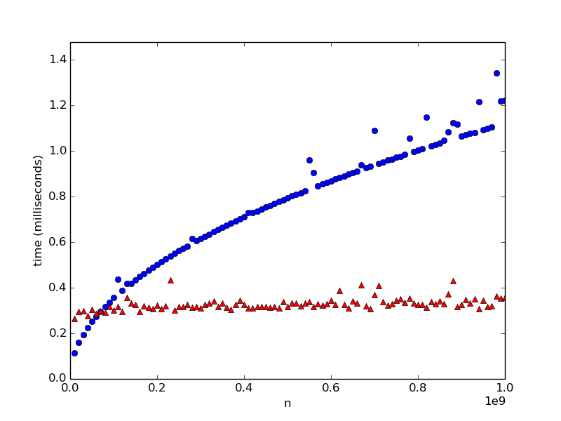
Quite a different picture, huh? In fact, for cryptographic purposes, we need to test prime numbers
that have hundreds or even thousands of digits. For numbers of that size, as it turns out,
the second algorithm
(which is called the Miller-Rabin primality testing algorithm) is the fastest way anyone knows how to
generate prime numbers. So even though it looked slower for the numbers that we initially tested on,
ultimately, is_prime2 is a far, far superior algorithm.
What happens if we run one of them on a different computer? Will we get the same times? Probably not — processor speed, operating system, memory, and a host of other things impact how much time it takes to execute a task.
Essentially, both algorihtms get slower as n increases, but algorithm 1 gets worse faster. And that will happen on any computer, and any reasonable implementation, in any programming language. How can we explain this behavior? And more importantly, how could we have predicted it without running the code?
2 Algorithm Analysis
Step counting
What we need, is a machine- and scenario-independent way to describe how much work it takes to run an algorithm. One thing that doesn't change from computer to computer is the number of basic steps in the algorithm (this is a big handwave, but generally true), so lets measure steps.
We are going to vaguely describe a "step" as a primitive operation, such as:
- assignment
- method calls
- arithmetic operation
- comparison
- array index
- dereferencing a pointer
- returning
It is important to note that this has a great degree of flexibility: one person's basic step is another person's multiple steps. To an electrical engineer, taking the not of a boolean is one step because it involves one bit. Adding two 32-bit numbers is 32 (or more!) steps. We won't be quite so anal.
So, when we determine how long an algorithm takes, we count the number of steps. More steps == more work == slower algorithm, regardless of the machine.
What does the following code do, and how many steps does it take?
1 2 3 4 5 6 7 | m = a[0]; # 2 steps: array lookup and assignment i = 1 # 1 step: assignment while i < n: # 1 comparison (each time) if a[i] > m: # 2: array and comparison m = a[i] # 2, but it doesn't always happen! i += 1 # 1 step, increment i return m # 1: we'll count calls and returns as 1. |
The loop gets executed exactly \(n-1\) times, and the loop condition
i < n happens one extra time when the loop terminates, so
the total number of steps is
\(2 + 1 + (n-1)(1 + (2\text{ or }4) + 1) + 1 + 1\).
Now, we're not quite done. In the code above, there are circumstances under which it will run faster than others. For example, if the array is in descending order, the code within the if statement is never run at all. If it is in ascending order, it will be run every time through the loop. We call these "best case" and "worst case" run times. We can also consider and talk about the "average" run time.
The best case is usually way too optimistic (most algorithms have best case times that are far away from average). Average case is often hard, because we need probabilistic analysis. In many cases, a worst case bound is a good estimate. That way we can always say, "no matter what, this program will take no more than this many steps." In the formula above, this means the \((2\text{ or }4)\) part just becomes 4.
Beginning of Class 4
Comparing algorithms with bounds
In the program above, the number of steps it takes depends on the size of the array, the n. What we really want is a function that takes the size of the array as input, and returns the number of steps as the output. Note that is what we developed above.
\(f(n) = 2 + 1 + (n-1)(1 + 4 + 1) + 1 + 1\), which simplifies to
\(f(n) = 6n - 1\).
So when we're comparing algorithms, we don't compare numbers, but functions. But how do we compare functions? Which function below is "bigger"?
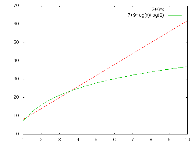
Well, sometimes one, and sometimes the other. So what we'll do is talk about one function dominating the other. We'll say that one function dominates another if it is always bigger than the other for every x value (for example \(f(x) = x^2\) dominates \(f(x)=-x^2\)). Neither of the functions in the graph above dominates the other.
One function can dominate another in a particular range as well. \(f(x)=1\) dominates \(f(x) = x^2\) in the range \([0;1]\).
Now, when input sizes are small, everything is fast. Differences in run time are most relevant when there is a lot of data to process. So, we colloquially ask "When n is large, does one dominate the other?" Mathematically, we ask if there exists an \(n_0\geq 1\) such that for all \(n\ge n_0\), \(f(n) \gt g(n)\) (or \(g(n) \gt f(n)\)).
In this graph, \(f(x)=3x^2-8\) dominates \(f(x)=x^2\) everywhere to the right of \(x=2\). So \(n_0=2\) - I like to call this the "crossover point".
How can we tell if one will dominate the other for large n?
It turns out it's really easy. It is all about growth rate. Take a look at this graph of \(f(n)= n^2\) vs. \(g(n) = 3n+4\).
What happens if we change the constants in \(g(n)\)? The line moves, but it doesn't change shape, so there's always some point at which f(n) passes it. Here for example is \(f(n)= n^2\) vs. \(g(n) = 30n+40\).
As soon as we start caring about really big n, it doesn't matter what the constant coefficients are, \(f(x)\) will always find a point at which it will dominate \(g(x)\) everywhere to the right. In the following table, \(f(n)\) will dominate \(g(n)\) for some large enough \(n\):
| \(f(n)\) | \(g(n)\) |
| \(n^2\) | \(n\) |
| \(n^2-n\) | \(5n\) |
| \(\frac{1}{10^{10}}n^2-10^{10} n - 10^{30}\) | \(10^{10} n + 10^{300}\) |
Big-O Notation
We talk about the runtime of algorithms by categorizing them into sets of functions, based entirely on their largest growth rate.
The mathematical definition: if two functions \(f(n)\) and \(f'(n)\) are both eventually dominated by the same function \(c\cdot g(n)\), where \(c\) is any positive coefficient, then \(f(n)\) and \(f'(n)\) are both in the same set. We call this set \(O(g(n))\) (pronounced "Big-Oh of g(n)"). Then we can write \(f(n) \in O(g(n))\) and \(f'(n) \in O(g(n))\).
Since the constant coefficients don't matter we say that \(g(n)\) eventually dominates \(f(n)\) if there is ANY constant we can multiply by \(g(n)\) so that it eventually dominates \(f(n)\). \(f(n)=5n+3\) is obviously \(O(n^2)\). It is also \(O(n)\), since \(f(n)\) is dominated by \(10n\), and 10 is a constant.
Beginning of Class 5
The formal definition:
\(f(n) \in O(g(n))\) if and only if there exist constants \(c\) and \(n_0\) such that \(c \gt 0\), \(n_0 \geq 0\), and for all \(n \ge n_0, f(n) \leq cg(n)\).
While \(f(n)=5n+10 \in O(n^2)\), it is also \(O(5n)\). \(O(5n)\) is preferred over \(O(n^2)\) because it is closer to \(f(n)\). \(f(n)\) is ALSO \(\in O(n)\). \(O(n)\) is preferred over \(O(5n)\) because the constant coefficients don't matter, so we leave them off.
Welcome to the Big-O club
We're a week in, and you've already learned the most important part of this class: Big-O notation. You absolutely have to understand this to speak intelligently about running time and complexity of computer programs. And we'll be using it quite a bit in this class.
Our Main Big-O Buckets and Terminology
Big-O is extremely useful because it allows us to put algorithms into "buckets," where everything in that bucket requires about the same amount of work. It's important that we use the correct terminology for these buckets, so we know what we're talking about. In increasing order...
- Constant time. The run time of these algorithms does not depend on the input size at all. \(O(1)\).
- Logarithmic time. \(O(\log(n))\). Remember, changing the base of the log is exactly the same as multiplying by a coefficient, so we don't tend to care too much if it's natural logarithm, base-2 logarithm, base-10 logarithm, or whatever.
- Linear time. \(O(n)\).
- n-log-n time. \(O(n \log(n))\).
- Quadratic time. \(O(n^2)\).
- Cubic time. \(O(n^3)\).
- Polynomial time. \(O(n^k)\), for some constant \(k\gt 0\).
- Exponential time. \(O(b^n)\), for some constant \(b \gt 1\). Note this is different than polynomial.
Beginning of Class 6
Fuzzily speaking, things that are polynomial time or faster, are called "fast," while things that are exponential, are "slow." There is a class of problems that are believed to be slow called the NP-complete problems. If you succeed in either (a) finding a fast algorithm to compute an NP-complete problem, or (b) prove that no such algorithm exists, congratulations! You've just solved a Millenium Problem, get a million dollars, and are super-famous. If you take the algorithms class, you'll learn how to do that.
The following table compares each of these buckets with each other, for increasing values of \(n\).
| \(n\) | \(\log(n)\) | \(n\) | \(n\log(n)\) | \(n^2\) | \(n^3\) | \(2^n\) |
| 4 | 2 | 4 | 8 | 16 | 64 | 16 |
| 8 | 3 | 8 | 24 | 64 | 512 | 256 |
| 16 | 4 | 16 | 64 | 256 | 4096 | 65536 |
| 32 | 5 | 32 | 160 | 1024 | 32768 | 4294967296 |
| 64 | 6 | 64 | 384 | 4096 | 262144 | 18446744073709551616 |
| 128 | 7 | 128 | 896 | 16384 | 2097152 | 340282366920938463463374607431768211456 |
| 256 | 8 | 256 | 2048 | 65536 | 16777216 | 115792089237316195423570985008687907853269984665640564039457584007913129639936 |
| 512 | 9 | 512 | 4608 | 262144 | 134217728 | 13407807929942597099574024998205846127479365820592393377723561443721764030073546976801874298166903427690031858186486050853753882811946569946433649006084096 |
| 1024 | 10 | 1024 | 10240 | 1048576 | 1073741824 | 179769313486231590772930519078902473361797697894230657273430081157732675805500963132708477322407536021120113879871393357658789768814416622492847430639474124377767893424865485276302219601246094119453082952085005768838150682342462881473913110540827237163350510684586298239947245938479716304835356329624224137216 |
To understand just how painful exponential time algorithms are, note that the number of seconds in the age of the universe has about 18 digits, and the number of atoms in the universe is a number with about 81 digits. That last number in the table has 309 digits. If we could somehow turn every atom in the universe into a little computer, and run all those computers in parallel from the beginning of time, an algorithm that takes \(2^n\) steps would still not complete a problem of size \(n=500\).
3 Big-O of Arrays and Linked Lists
Analyzing Data Structures we already know
We are already quite comfortable with two types of data structures: arrays, and linked lists (we also know array lists, but those require some more complicated analysis). Today we're going to apply our analysis skills to the operations we commonly do with these data structures.
Access
"Access" means getting at data stored in that data structure. For example, getting the third element.
In an array, this is really easy! theArray[3] Does the time this takes depend upon the size of the array? No! So, it's constant time. \(O(1)\).
In a Linked List, this is harder. Now, if we were looking for the first element, or the third element, or the hundredth element, then that does NOT depend upon the size of the list, and that would be \(O(1)\). However, remember that we are interested in worst case, and our adversary gets to choose which element we want. So, of course, he would choose the last one. This requires that we cycle through every link in the list, making it \(O(n)\).
Adding an Element to the Front or Back
In an array, this is hard! Because we now have an additional element to store, we have to make our array bigger, requiring us to build a new array of size n+1, move every element into it, and add the new one. That "move every element into it," will take \(O(n)\) time.
In a linked list, this is really easy! If we have a pointer to the first and last link in the chain, this takes the same amount of time, no matter how long the list is! \(O(1)\).
It's worth noting that removing an element requires a similar process.
Adding an Element to a Sorted List or Array
The scenario: assume the array or list is in sorted order, and we have a new element to add. How long will it take (as always, in the worst case)?
This is a two-step process: (1) find where the element goes, and (2) add the element.
In arrays, we recently saw two ways to do (1); one where we cycled through the entire array looking for the proper location (\(O(n)\), and one where we repeatedly halved the array until we found the spot (this is called binary search, and takes \(O(log(n))\)). Doing step (2) is very similar to what we had to do for adding an element to the front or back, so that step is \(O(n)\). So, in total, this takes us \(O(log(n)) + O(n)\), which is \(O(n)\).
Alternatively, you could skip binary search, and do a sequential search (go from element to element, front to back until you find it), moving elements to the new array as you go. Once you find the location to add your new element, add it to the new array, and continue moving elements. This gives you two loops, each of which move roughly half the array. Again, in total, this gives us \(O(n)\).
In a linked list, doing step (1) is \(O(n)\) (see why?). Adding the element at that point is \(O(1)\). So, in total, \(O(n)\).
In summary, it's \(O(n)\) for either an array or a linked list. But there's a big difference in how this breaks down. For arrays, the \(O(n)\) really comes from the "insertion" part, whereas for linked list the insertion part is easy and the \(O(n)\) comes from the "search" part. This difference will come into play in some applications later on.
Traversal
Traversal is our word for "visiting every element." It should be clear that for both arrays and linked lists, this is \(O(n)\).
Why did we do this?
The executive summary is as follows:
| Array | Linked List | |
| Access | \(O(1)\) | \(O(n)\) |
| Insertion or removal from front or back | \(O(n)\) | \(O(1)\) |
| Sorted insertion or removal | \(O(n)\) | \(O(n)\) |
| Traversal | \(O(n)\) | \(O(n)\) |
We'll be doing this all semester, for each of our data structures. As you can see, the choice between arrays and linked lists, comes down to what you're doing with them. Doing lots of access? Use an array. Adding and removing elements often? Use a linked list. This give-and-take is at the center of Data Structures.