Credit: Gavin Taylor for the original version of these notes.

1 Graph Basics

Graphs aren't new to us. Remember that a graph is a set of vertices, and the edges that connect them. We remember this because we've been dealing with trees, and trees, as we learned, are just a special form of graph.

Graphs are a spectacularly useful mathematical construct, and a lot of seemingly unrelated problems can be viewed as graph problems. This is a useful thing to have, because if somebody can solve a general graph problem, then they've solve every application that somebody can get to look like a graph problem.

What are some examples of graphs? Here's the DC Metro system:

The map of the Metro is a graph where Metro stops are the vertices, and the routes the trains take are the edges.

We could also draw the friendships in a social network as a graph:

Finally, we have a drawing of the proposed ARPANET in the late 1960s:

There are a lot of questions we can ask about these types of relationships: What is a route between Suitland and Foggy Bottom (I think we can agree those are the two silliest Metro station names)? Does Jack know Jill? Does Jack know somebody who knows Jill?

All of these graphs are undirected, which means that the pathways run both ways: people are friends with each other, and a path between New Carrollton and Landover implies a path between Landover and New Carollton. But, they don't have to be. Google represents the internet using a directed graph: a directed edge between two pages P1 and P2 exists if P1 links to P2.

Simplistically speaking, Google calculates the probability of ending up at a certain page given random clicks (equating to a random walk around the graph). The higher the probability that you end up on a page, the more influential and important it is.

So those two graphs are directed, but they are all still unweighted. Consider this graph:

In this graph, the edges are weighted by the amount of time it takes to get between different places. If I'm home, and need to go to work, the grocery store, and the gas station, what's the fastest path?

So graph algorithms are really, really important, and we'll be spending some time on them.

2 Graph terminology

• Undirected Graph: Graph in which all edges are undirected.
• Directed Graph: Graph in which all edges are directed.
• Weighted graph: The edges are associated with a numerical value.
• Adjacent Vertices: Vertices connected by an edge.
• Degree: The number of edges connected to a vertex is its degree. If there are \(m\) edges in a graph, \(\sum_{v\in G} deg(v) = 2m\) (because each edge is connected to two vertices).
• In degree and out degree: Number of directed edges coming into or going out of a vertex.
• Path: A sequence of vertices, such that each vertex is adjacent to the vertices preceding and succeeding it.
• Two vertices are connected if there is a path that goes from one to the other.

There are also some variable names that are used pretty consistently, so let's write them down here so we can all get on the same page:

• \(u, v\): usually the names of vertices
• \(w\): usually the weight of some edge
• \(V\): the set of all vertices
• \(E\): the set of all edges
• \(G\): a complete graph, which is just a pair \((V,E)\).
• \(n\): the number of vertices in the graph
• \(m\): the number of edges in the graph

3 Graph ADT

The precise interface for dealing with a graph will depend slightly on whether it's weighted or unweighted, and directed or undirected. We'll describe an abstract data type for a directed and weighted graph; it might be just a little bit simpler if the graph doesn't have directions or weights.

• getVertices(): returns a list of all vertex labels in the graph
• getEdge(u, v): returns the weight of the edge from u to v, or null if there is no such edge
• neighbors(u): returns a list of edges that start from the vertex labeled u
• addVertex(u): adds a new vertex labeled u, which will initially have no neighbors
• addEdge(u, v, w): adds a new edge from u to v with weight w

4 Representing a Graph

Now we have a graph ADT, so what will the data structures be to implement that ADT? Well there are actually two things to represent here: the vertices, and the edges.

To represent the vertices, we need a Map that will associate any vertex name (probably a string, but maybe something else) to that vertex's representation in the data structure. So the keys in this map will be vertex labels. The best choices would be a balanced search tree or a hashtable.

What will the "representation in the data structure" for each vertex be? Well that depends on how we are storing the edges. First, you can use an adjacency list. In an adjacency list, each vertex is an object which contains a list of edges going out from that vertex. (And each edge object should have the vertex names that it goes from and towards, as well as its weight where applicable.) In the case of an adjacency list, your vertex map would have labels as the keys and vertex objects as the values.

The second option is an adjacency matrix. In this, if we have \(n\) vertices, we construct a \(n \times n\) matrix using a double array. Each vertex is simply represented by an index from 0 to \(n-1\), so that every vertex has a row and a column dedicated to it. If location \((i,j)\) is null, no edge connects \(V_i\) and \(V_j\). If an edge does connect those two vertices, location \((i,j)\) will be a pointer to that edge. Alternatively, you could quit on creating Edge objects, and have the matrix be boolean, true if an edge exists, and false otherwise. For a weighted graph, the weight could be stored in that location.

Again, going from a vertex to an index in the matrix requires a map, mapping vertices to indices.

There must be pros and cons to each of these. Let's call the number of vertices \(n\), and the number of edges \(m\).

• Space: For an adjacency list, there are \(n\) independent lists, so you may want to say this is \(O(n)\), because we've never considered anything other than \(n\) in our function. However, the sparsity of the graph (ie, the number of edges), changes the amount of space required. If there are a lot of edges, each vertex's list is substantial; if there are few, each list is small. So, an adjacency list requires \(O(m+n)\) space. An adjacency matrix, on the other hand, has an entry for each possible edge, whether it exists or not. So, an adjacency matrix requires \(O(n^2)\) space. Which is bigger? Depends on the graph!
• getVertices(). This is a simple traversal through the map, which should always be \(O(n)\).
• getEdge(u,v), i.e., testing whether a certain edge exists. First we have to look up u and v in the map. Then, in an adjacency matrix the edge is just an entry in the double array, \(O(1)\) time to look it up. In an adjacency list, the cost depends on how many neighbors u has, so it's \(O(\deg u)\), which could be as much as \(O(n)\).
• neighbors(u), i.e., returning a list of all vertices incident to a vertex u: For an adjacency list, this list already exists, you merely have to return a pointer to it. So, this is (time to get the vertex's list in the map) + \(O(1)\). For an adjacency matrix, this list has to be created, and each vertex has to be checked to see if it belongs in there: (time to get the vertex's index)+\(O(n)\).
• addVertex(u):, i.e., inserting a vertex: For the adjacency list, this merely requires adding a new vertex to the list of vertices. The runtime of this depends upon your map (\(O(1)\) for a hashtable, \(O(\log(n))\) for a tree, etc.). For the adjacency matrix, you have to add a new row and column to the matrix: \(O(n)\) amortized. (Because sometimes the underlying arrays will have to be doubled in size, costing \(O(n^2)\) in the worst case.)
• addEdge(u,v,w), i.e., inserting an edge: For both, this is pretty easy. You have to start by looking up both vertex labels in the map. Then you either add something to the linked list, or set an entry in the matrix. Both of those last steps are \(O(1)\).

5 Depth-First Search

One of the things we want to do with just about any data structure is traverse it, meaning to iterate over all the things in that data structure in some kind of order. We talked about 4 different ways to traverse trees; what changes when we want to traverse a graph instead?

The first thing that changes is the name: traversing a graph is called graph search as it is "exploring" the graph in some way. And while tree traversals always start from the root, a graph search can start from anywhere. So a graph search always has a particular starting vertex; it might have an ending (or "destination") vertex too, like if we are searching for a particular path through the graph.

If we took the usual pre-order traversal algorithm from trees and applied it to graphs, it would work except for one small problem: any cycle in the graph would result in an infinite loop in the algorithm! So we have to add one more thing, a map visited which stores T/F for each node depending on whether that node has already been visited.

The pseudocode for this search might look something like this:

1
2
3
4
5
6
7
8
9
10
11
12

DFS(G, start):
    visited = new Map from vertices to T/F
    DFS(G, start, visited)
 
DFS_Helper(G, uu, visited):
    if visited.get(uu) == true:
        return
    else:
        visited.set(uu, true)
        print(uu.data)
        for each node vv in G.neighbors(uu):
            DFS_Helper(G, vv, visited)

This is called a Depth-First-Search, or DFS for short, because of the way it explores the graph; it sort of "goes deep" before it "goes wide".

That's a mighty fine recursive algorithm, but of course we could write it iteratively too if we wanted. The main difference is that we will need a stack to store the nodes that are currently being explored. This essentially takes the place of the function call stack that the recursion uses without thinking.

1
2
3
4
5
6
7
8
9
10
11
12
13

DFS(G, start):
    visited = new Map from vertices to T/F
    fringe = new Stack of vertices
 
    fringe.push(start)
    while fringe is not empty:
        uu = fringe.pop()
 
        if visited.get(uu) != true:
            visited.set(uu, true)
            print(uu.data)
            for each node vv in G.neighbors(uu):
                fringe.push(vv)

DFS is great when we are trying to just traverse the graph and we don't care about the order, or if we are trying to learn somethinig about cycles or ordering relationships in a directed graph. For example, if you had a graph and wanted to know whether or not it contained any cycles, you could do a DFS starting from each vertex, and check if each child node vv is already in the fringe before adding it on the last line. If we come across a node in the neighbors of uu that is already in the stack, then we've found a cycle in the graph!

6 Breadth-First Search

Let's go crazy and replace the stack from DFS with a queue instead. What happens is that we get something more like a level-order traversal of a tree, where the nodes closest to the starting vertex are explored first. This is called a breadth-first search (BFS), and it can be used to find the shortest path between two vertices in an unweighted graph.

Here's pseudocode for BFS, where we also added in a map of "parents" that keeps track of the shortest paths, for purposes of backtracking and recovering that actual path later.

1
2
3
4
5
6
7
8
9
10
11
12
13
14
15
16
17
18

BFS(G, start):
    visited = new Map from vertices to T/F
    fringe = new QUEUE of vertices
    parent = new Map from vertices to vertices
 
    fringe.enqueue(start)
    while fringe is not empty:
        uu = fringe.dequeue()
        print(uu.data)
 
        if visited.get(uu) != true:
            visited.set(uu, true)
            print(uu.data)
 
            for each node vv in G.neighbors(uu):
                if visited.get(vv) != true:
                    parent.set(vv, uu)
                    fringe.enqueue(vv)

Note that if there was a particular destination vertex we were searching for, the BFS could be terminated as soon as we find that vertex on line 15. Recovering the path is just a matter of following the vertices in parent until you get back to the start.

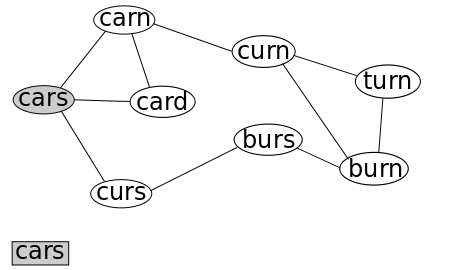
Here's an example of this running, where I use an old WordLadder project to demonstrate. Here, each vertex is an English word, and if two words are exactly one letter apart (like "cape" and "cane"), then an edge is drawn between then. We're searching for a path from "cars" to "turn."

We will mark nodes as being "visited" by greying them out, and will mark a node's parent by drawing a red arrow. The Queue is illustrated just below the graph.

We start by adding "cars" to the Queue, and marking it as "visited."

We now remove the first node in our Queue, which is, of course "cars", and add each connected, non-visited node to the Queue, noting that their parents are "cars."

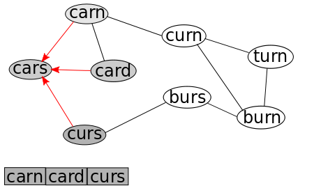
We now repeat this: we remove the first node in our Queue, which is now "carn", and add each connected, non-visited node to the Queue (there are three connected nodes, but two have already been visited), noting that their parents are "carn."

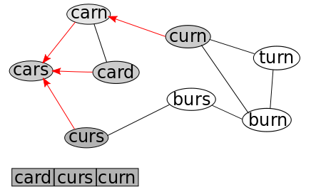
This time when we remove the first node in the Queue, it has ZERO connected, non-visited nodes. So the only effect is "card" is removed from the queue.

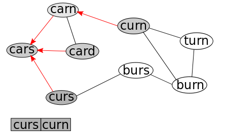
Repeating this process now results in the removal of "curs" from the Queue, and the addition of its only connected, non-visited node, "burs." As always, we mark "burs" as visited, and note that its parent is "curs."

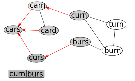
We repeat this, by removing "curn" from the Queue, and looking at its connected, non-visited nodes, one of which is actually our target node! So, we're done, but what now?

Now, the parent notations become useful; we can now walk them back and see the path we took through the graph. turn-> curn-> carn-> cars. Success!

Essentially, this works by adding all vertices that are one step away from u to the queue, then all the vertices two steps away, then three.

So, what does BFS guarantee us? Well, first, the only thing that causes this to stop, is we either find v, or we run out of connected, unvisited vertices. So, if a path exists (if v is connected to u), then we are guaranteed to find it. Additionally, because all vertices that can be reached in \(k\) steps are added before any vertices that can only be reached in \(k+1\) steps are added, the path we find will be the shortest such path that exists. Cool!

Credit Randall Munroe, XKCD.com

It's worth noting that the BFS and DFS algorithms don't change if we're looking at a directed graph.

7 Runtime of graph search

The runtime for both algorithms depends on the implementation of the Graph (adjacency list or adjacency map) and the implementation of the map therein. When done the fastest possible way, with a HashMap and an Adjacency List, this costs \(O(m+n)\), where \(m\) is the number of edges, and \(n\) is the number of vertices.

Though this is a good fact to know, it's more important that you be able to derive this runtime from the pseudocode above.