Unit 5: Maps
Credit: Gavin Taylor for the original version of these notes.
Beginning of Class 16
1 Maps
Maps
It's time for a new ADT: the Map. Every piece of data in a Map has two parts: a key and an associated value. Sometimes this is called a key-value pair. We find the value, by searching for the key. For example, a dictionary is a map: we look up the word (the key), and get the definition (the value). In fact, in some textbooks they use the word Dictionary for the Map ADT.
A phone book is a Map too: we look up the name, and get the phone number and address. In IC210, maybe you did a lab where you counted how many times words appeared in a document; the word was the key, and the count was the value. The important thing is that the keys be sortable (like numbers, or strings), so that we can be smart about storing them.
Suppose we were interested in creating a system to look up a mid's grades, which wasn't as terrible as MIDS. First, you might make a class that can contain all of a single student's grades (we'll call it Grades, because we're creative). Then, you want it to be searchable by alpha.
Operations of a Map
The operations are:
get(key): Returns the value associated with the given key, ornullif it's not in the map.set(key, value): Inserts a new key-value pair into the map, or changes the value associated with the given key if it's already in the map.size(): Returns the number of distinct keys that are stored in the map.
You may be wondering about a few things here. First, why are we using
null as a special "sentinel" value to indicate something is not
found in the map? Isn't that bad style? Well maybe it is, but this is how
some of Java's built-in methods behave, and it allows us to make the Map
interface much simpler and avoid having to deal with too many exceptions.
(The only downside is that you are not allowed to store null values in a map.)
You may also be wondering why there's no remove method. Well,
to remove something, you just set its value to null! The underlying
Map implementation can either choose to actually remove that part of the
data structure in that case, or it could just store null as the
value and no one would be the wiser!
In general, in this class, we're going to avoid talking about how removal from
Maps works, not because it can't be done, but because it's not strictly
necessary and this way we can cover a greater variety of data structures.
We're going to spend a lot of time on Maps, implementing them with new data structures. For now, a map can be implemented with an array (either in sorted order by key, or unsorted), a linked list (again, either sorted by key, or unsorted), or Binary Search Tree (organized by key). Note that a Node in a LL or BST will now contain not a single data field, but both the key and the element. For an array, you would need to combine the key and element together into a single object, like the one below.
1 2 3 4 5 6 7 8 9 10 11 12 13 14 15 16 17 18 19 | public class AlphaGradePair implements Comparable<AlphaGradePair> { private int alpha; private Grade daGrade; public AlphaGradePair(int alpha, Grade daGrade) { this.alpha=alpha; this.daGrade=daGrade; } public int getKey() { return alpha; } public Grade getGrade() { return daGrade; } public int compareTo(AlphaGradePair other) { if (alpha < other.getKey()) return -1; else if (alpha > other.getKey()) return 1; else return 0; } } |
How would you implement these methods for each of these data structures?
| set(k,e) | get(k) | |
|---|---|---|
| Unsorted array | O(1) (amortized) | O(n) |
| Sorted array | O(n) | O(log(n)) |
| Unsorted Linked List | O(1) | O(n) |
| Sorted Linked List | O(n) | O(n) |
| Binary Search Trees | O(height) | O(height) |
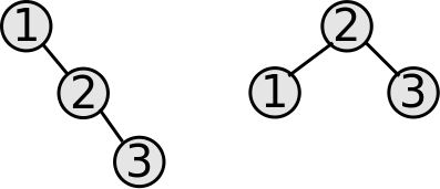
For now, we know that the height of a tree is somewhere between log(n) and n. If only we had a way to guarantee the tree would be balanced! If only...
Beginning of Class 17
2 AVL Trees
AVL Trees
We're going to learn about two types of self-balancing trees in this class, defined as "trees that always meet some definition of balanced." There's a wide variety of these, and I think they're pretty cool.
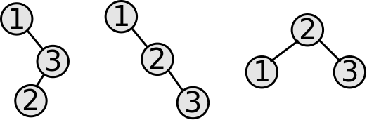
AVL Trees define "balanced" as "the heights of the subtrees of any node can differ by at most one." Note, this is NOT the same as "the tree is as short as possible." For example, consider this tree:
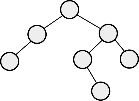
This tree is NOT complete (meaning totally filled in). However, by the definition of AVL trees, it IS balanced. The height of an AVL tree is still \(O(\log(n))\).
Rotations
AVL trees keep themselves balanced by performing rotations. A tree rotation is a way of rearranging the nodes of a BST that will change the height, but will NOT change the order. That's really important - the nodes in a BST are always in order, before and after every rotation operation. All that we change is the levels of some of the nodes to fix up the height.
The following illustration demonstrates a left rotation on the root node, x:
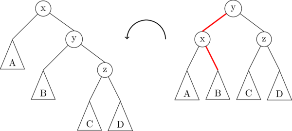
In this illustration, the triangles A, B, C, D represent subtrees which might be empty (null), or they might contain 1 node, or a whole bunch of nodes. The important thing is that the subtrees don't change, they just get moved around. In fact, there are only really two links that get changed in a right rotation; they are highlighted in red in the image above.
Pseudocode for a left rotation is as follows:
1 2 3 4 5 6 7 | Node lRotate(Node oldRoot) { // oldRoot is node "x" in the image above. Node newRoot = oldRoot.right; // newRoot is node "y" in the image above. Node middle = newRoot.left; // middle is the subtree B newRoot.left = oldRoot; oldRoot.right = middle; return newRoot; } |
A right rotation on the root node is exactly the opposite of a left rotation:
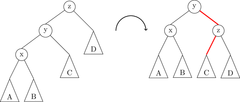
To implement rRotate, you just take the code for lRotate, and swap right and left!
Adding to an AVL tree
The idea that makes AVL trees possible to quickly implement is that nodes are modified to include the height of the subtree rooted at that node. An empty tree (null) has a height of -1, leaves have a height of 0, and any other node \(u\) has a height of \(1 + \max(u.left.height, u.right.height)\).
We also define balance, where balance = n.right.height-n.left.height.
If, at any point, balance becomes -2 or 2, we must perform at least one rotation to rebalance the tree. There are four cases to consider:
(balance(uu) == 2 && balance(uu.right) >= 0) Left rotate at the root.
(balance(uu) == 2 && balance(uu.right) == -1) Right rotate at the right subtree, then left rotate at the root. (This is called a "double rotation").
The other two cases are the mirror images of the above two.
Getting an element of an AVL Tree
This is no different from find or get in any other binary search tree!
Beginning of Class 18
Height of an AVL tree
So far, we know that we can implement the Map ADT with an AVL tree, which is
a special kind of BST which maintains a balance property at every node.
And we know that the cost of get and set in a BST
is \(O(height)\). If you think about it, each AVL rotation operation is
\(O(1)\), and so even in an AVL tree, the get and set
operations are \(O(height)\).
What makes AVL trees useful is that, unlike any old Binary Search Tree, the height of an AVL tree is guaranteed to be \(O(log n)\), where \(n\) is the number of nodes in the tree. That's amazing! Here's how you prove it:
Let's write \(N(h)\) to be the minimum number of nodes in a height-\(h\) AVL tree. Remember that we know two things about an AVL tree: its subtrees are both AVL trees, and the heights of the subtrees differ by at most 1. And since the height of the whole tree is always one more than one of the subtree heights, the balance property means that both subtrees have height at least \(h-2\).
Now since both subtrees have height at least \(h-2\), and both of them are also AVL trees, we can get a recurrence relation for the number of nodes:
\[N(h) = \begin{cases} 0,& h=-1 \\ 1,& h=0 \\ 1 + 2N(h-2),& h\ge 1 \end{cases}\]This isn't a recurrence for the running time of a recursive function, but it's a recurrence all the same. That means that we know how to solve it! Start by expanding out a few steps:
\[\begin{align*} N(h) &= 1 + 2N(h-2) \\ &= 1 + 2 + 4N(h-4) \\ &= 1 + 2 + 4 + 8N(h-6) \end{align*}\]You can probably recognize the pattern already; after \(i\) steps, it's
\[N(h) = 1 + 2 + 4 + \cdots + 2^{i-1} + 2^i N(h-2i)\]We know that the summation of powers of 2 is the next power of 2 minus 1, so that can be simplified to
\[N(h) = 2^i - 1 + 2^i N(h-2i)\]Next we solve \(h-2i \le 0\) to get to the base case, giving \(i=\tfrac{h}{2}\). Plugging this back into the equation yields:
\[N(h) = 2^{h/2} - 1 + 2^{h/2} N(0) = 2^{h/2 + 1} - 1\]Hooray - we solved the recursion! But what now? Remember that \(N(h)\) was defined as the least number of nodes in a height-\(h\) AVL tree. So we basically just got an inequality relating the number of nodes \(n\) and the height \(h\) of an AVL tree:
\[n \ge 2^{h/2+1} - 1\]Solve that inequality for \(h\) and you see that
\[h \le 2\lg(n+1) - 2\]And wouldn't you know it, that's \(O(log n)\).
Beginning of Class 19
3 2-3-4 Trees
Our next self-balancing tree is called a 2-3-4 tree (or a B-tree of order 4), so called because nodes can have anywhere from two to four children. Regular binary search trees can't always be perfectly balanced - that's why AVL trees have to allow the flexibility that subtree heights can differ by at most 1.
But because 2-3-4 trees allow nodes to have 2, 3, or 4 children, they can always be perfectly balanced! In other words:
Nodes in a 2-3-4 tree can contain multiple pieces of data, but the rules stay similar to a binary search tree; things to the right are bigger than things to the left. The nodes look like this:
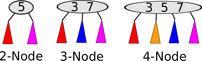
In the above image, in the 2-node, the red subtree consists of data smaller than 5, and the purple data consists of data larger than 5. In the 3-node, red data is smaller than 3, blue is between 3 and 7, and purple is larger than 7. In the 4-node, red is smaller than 3, yellow is between 3 and 5, blue is between 5 and 7, and purple is larger than 7. In summary:
- A 2-node has 1 key and 2 children.
- A 3-node has 2 keys and 3 children.
- A 4-node has 3 keys and 4 children.
In general, the number of children of any node has to be exactly 1 more than the number of keys in that node. The keys in a node go "between" the keys of each child subtree.
Splitting a 4-node
Just like rotations were the key operation to keeping an AVL tree balanced, node split operations are the key to maintaining a balanced 2-3-4 tree when we do additions. Here's how splitting works:
- Only a 4-node can be split.
- The smallest key and the two smallest children form a new 2-node.
- The largest key and the two largest children form a second new 2-node.
- The middle key goes into the parent node (it gets "promoted"), and the new 2-nodes are new children of the parent node.
For example, given the following 4-node:

it would be split as follows:

In that image, the (x) and (z) nodes are newly-created 2-nodes, and the (y) would be inserted into the parent node. If there is no parent node, meaning that (x,y,z) was the root node before, then (y) becomes the new root node.
Adding to a 2-3-4 Tree
The algorithm for insertion is dead-simple, once you understand how to split. What makes it easy is that we follow this rule: you never insert into a 4-node. Whenever you encounter a 4-node that you might want to insert into, you split it first! Here's an example:

Let's first try to insert 18:

That was easy! There were no 4-nodes along the way, so no splits needed and we just put 18 in the leaf node where it belongs.
Now let's keep going and insert 60:

See what happened? The search for 60 ended up in the 4-node (33,40,52). Since we can't insert into a 4-node, we split that node first and promoted 40 to the top level before proceeding to insert 60 below.
Keep going: insert 79:

That time, two splits were necessary in order to do the insertion. Since we split the root node, we got a new root node (and the height of the tree increased by 1).
So how long does an insert take? Well, in the best case, all the nodes along the search path are 2-nodes or 3-nodes, so we can just add the new value to an existing leaf node. That takes \(O(\log n)\), since the height of a 2-3-4 tree is always \(O(\log n)\).
In the worst case, we have to split at every level down to the leaf. But each split is a constant-time operation, so the cost in the worst case is still \(O(\log n)\)! Therefore the cost of get or set in a 2-3-4 tree is \(O(\log n)\).
Implementation
So how do we implement this? Well... you probably don't. There's another balanced BST called a Red-Black Tree which is equivalent to a 2-3-4 tree, but where every 2-3-4 node is turned into 1, 2, or 3 BST nodes that are either colored "red" or "black". People tend to use red-black trees as the implementation because some of the rules for balancing are easier to implement, particularly when you want to remove something from the tree. (In the linked-to Wikipedia article, check out the section called "Analogy to B-trees of order 4").
If you're implementing your own balanced tree, you might want to choose to look up a Red-Black tree and do it that way. However, you are not required to know anything about them for this course.
Comparison to AVL Tree
The tallest a 2-3-4 tree would be one made up entirely of 2-nodes, making it just a binary search tree. But since 2-3-4 trees are always perfectly balanced, the height in that worst case would still be \(O(\log n)\), comparable to AVL trees. But, which is better?
As is often the case, the answer is "it depends." 2-3-4 trees have balanced height, but can have rather unbalanced weight. That is, the height of all subtrees will be the same, but the number of keys in each subtree could differ by a factor of two or more.
This makes the running time potentially slower for 2-3-4 trees, because each get or set operation requires more comparisons that an AVL tree would. However, the memory usage is better because there are fewer nodes and hence fewer pointers that must be stored.